
全网最全!国赛一等奖作品!代码+模型+结果2 0 2 5 年 第 五 届 长 三 角 高 校 数 学 建 模 竞 赛赛题 B:空气源热泵供暖的温度预测,关注我,持续分享!需要全文内容请关注
关注我,持续分享!需要全文内容请关注!
2 0 2 5 年 第 五 届 长 三 角 高 校 数 学 建 模 竞 赛
赛题 B:空气源热泵供暖的温度预测
问题 1 统计所给不同建筑的室内温度波动规律;绘制室内外温度相关性曲线, 分析热泵能耗与温差的定量关系;分析影响室内温度的影响因素。
1.结果
读取地点1数据...
成功读取地点1数据,共57512条记录
原始数据列名: ['设备编码', '采集时间', '测点温度(℃)', '采集点', '年份', '文件名', '时 间']
处理后数据列名: ['时间', '采集点', '年份', '室内温度', '小时', '日期', '月份', '星期', '是否夜间']
数据预处理完成,共57512条有效记录
地点1室内温度波动规律分析
室内温度基本统计量:
count 57512.000000
mean 20.371347
std 1.973280
min -13.700000
25% 19.400000
50% 20.500000
75% 21.600000
max 28.600000
Name: 室内温度, dtype: float64
地点1影响室内温度的因素分析
Traceback (most recent call last):
File "anaconda3\Lib\site-packages\patsy\compat.py", line 36, in call_and_wrap_exc
return f(*args, **kwargs)
^^^^^^^^^^^^^^^^^^
File "anaconda3\Lib\site-packages\patsy\eval.py", line 169, in eval
return eval(code, {}, VarLookupDict([inner_namespace]
^^^^^^^^^^^^^^^^^^^^^^^^^^^^^^^^^^^^^^^^^^^^^^
File "<string>", line 1, in <module>
NameError: name '室外温度' is not defined
The above exception was the direct cause of the following exception:
Traceback (most recent call last):
File "5.15长三角数学建模\2025年第五届长三角高校数学建模竞赛赛题\2025年第五届长三角高校数学建模竞赛赛题\2025长三角赛题B:空气源热泵供暖的温度预测\temperature_analysis.py", line 572, in <module>
main()
File "5.15长三角数学建模\2025年第五届长三角高校数学建模竞赛赛题\2025年第五届长三角高校数学建模竞赛赛题\2025长三角赛题B:空气源热泵供暖的温度预测\temperature_analysis.py", line 531, in main
location1_factor_model = analyze_influencing_factors(location1_processed, "地点1")
^^^^^^^^^^^^^^^^^^^^^^^^^^^^^^^^^^^^^^^^^^^^^^^^^^^^^^^^^
File "5.15长三角数学建模\2025年第五届长三角高校数学建模竞赛赛题\2025年第五届长三角高校数学建模竞赛赛题\2025长三角赛题B:空气源热泵供暖的温度预测\temperature_analysis.py", line 394, in analyze_influencing_factors
model = ols('室内温度 ~ 室外温度 + 是否夜间 + C(月份) + C(小时)', data=df).fit()
^^^^^^^^^^^^^^^^^^^^^^^^^^^^^^^^^^^^^^^^^^^^^^^^^^^^^^^^^^^^^^^^^^
File "anaconda3\Lib\site-packages\statsmodels\base\model.py", line 203, in from_formula
tmp = handle_formula_data(data, None, formula, depth=eval_env,
^^^^^^^^^^^^^^^^^^^^^^^^^^^^^^^^^^^^^^^^^^^^^^^^^^^^^^^^
File "anaconda3\Lib\site-packages\statsmodels\formula\formulatools.py", line 63, in handle_formula_data
result = dmatrices(formula, Y, depth, return_type='dataframe',
^^^^^^^^^^^^^^^^^^^^^^^^^^^^^^^^^^^^^^^^^^^^^^^^^^^^^
File "anaconda3\Lib\site-packages\patsy\highlevel.py", line 309, in dmatrices
(lhs, rhs) = _do_highlevel_design(formula_like, data, eval_env,
^^^^^^^^^^^^^^^^^^^^^^^^^^^^^^^^^^^^^^^^^^^^^^^^^^
File "anaconda3\Lib\site-packages\patsy\highlevel.py", line 164, in _do_highlevel_design
design_infos = _try_incr_builders(formula_like, data_iter_maker, eval_env,
^^^^^^^^^^^^^^^^^^^^^^^^^^^^^^^^^^^^^^^^^^^^^^^^^^^^^^^^^^^
File "anaconda3\Lib\site-packages\patsy\highlevel.py", line 66, in _try_incr_builders
return design_matrix_builders([formula_like.lhs_termlist,
^^^^^^^^^^^^^^^^^^^^^^^^^^^^^^^^^^^^^^^^^^^^^^^^^^
File "anaconda3\Lib\site-packages\patsy\build.py", line 693, in design_matrix_builders
cat_levels_contrasts) = _examine_factor_types(all_factors,
^^^^^^^^^^^^^^^^^^^^^^^^^^^^^^^^^^
File "anaconda3\Lib\site-packages\patsy\build.py", line 443, in _examine_factor_types
value = factor.eval(factor_states[factor], data)
^^^^^^^^^^^^^^^^^^^^^^^^^^^^^^^^^^^^^^^^
cat_levels_contrasts) = _examine_factor_types(all_factors,
^^^^^^^^^^^^^^^^^^^^^^^^^^^^^^^^^^
File "anaconda3\Lib\site-packages\patsy\build.py", line 443, in _examine_factor_types
value = factor.eval(factor_states[factor], data)
^^^^^^^^^^^^^^^^^^^^^^^^^^^^^^^^^^^^^^^^
^^^^^^^^^^^^^^^^^^^^^^^^^^^^^^^^^^
File "anaconda3\Lib\site-packages\patsy\build.py", line 443, in _examine_factor_types
value = factor.eval(factor_states[factor], data)
^^^^^^^^^^^^^^^^^^^^^^^^^^^^^^^^^^^^^^^^
File "anaconda3\Lib\site-packages\patsy\build.py", line 443, in _examine_factor_types
value = factor.eval(factor_states[factor], data)
^^^^^^^^^^^^^^^^^^^^^^^^^^^^^^^^^^^^^^^^
ne_factor_types
value = factor.eval(factor_states[factor], data)
^^^^^^^^^^^^^^^^^^^^^^^^^^^^^^^^^^^^^^^^
value = factor.eval(factor_states[factor], data)
^^^^^^^^^^^^^^^^^^^^^^^^^^^^^^^^^^^^^^^^
^^^^^^^^^^^^^^^^^^^^^^^^^^^^^^^^^^^^^^^^
File "anaconda3\Lib\site-packages\patsy\eval.py", line 568, in eval
return self._eval(memorize_state["eval_code"],
^^^^^^^^^^^^^^^^^^^^^^^^^^^^^^^^^^^^^^^
File "anaconda3\Lib\site-packages\patsy\eval.py", line 551, in _eval
return call_and_wrap_exc("Error evaluating factor",
^^^^^^^^^^^^^^^^^^^^^^^^^^^^^^^^^^^^^^^^^^^^
File "anaconda3\Lib\site-packages\patsy\compat.py", line 43, in call_and_wrap_exc
exec("raise new_exc from e")
File "<string>", line 1, in <module>
patsy.PatsyError: Error evaluating factor: NameError: name '室外温度' is not defined
室内温度 ~ 室外温度 + 是否夜间 + C(月份) + C(小时)
^^^^
PS 5.15长三角数学建模\2025年第五届长三角高校数学建模竞赛赛题\2025年第五届长三角高校数学建模竞赛赛题\2025长三角赛题B:空气源热泵供暖的温度预测> & C:/Users/Jack/anaconda3/python.exe e:/小猪不爱学习/jiedan/5.15长三角数学建模/2025年第五届 长三角高校数学建模竞赛赛题/2025年第五届长三角高校数学建模竞赛赛题/2025长三角赛题B:空 气源热泵供暖的温度预测/temperature_analysis.py
开始分析空气源热泵供暖的温度数据...
读取地点1数据...
成功读取地点1数据,共57512条记录
原始数据列名: ['设备编码', '采集时间', '测点温度(℃)', '采集点', '年份', '文件名', '时 间']
处理后数据列名: ['时间', '采集点', '年份', '室内温度', '小时', '日期', '月份', '星期', '是否夜间']
数据预处理完成,共57512条有效记录
地点1数据中缺少室外温度信息,将使用模拟数据
地点1室内温度波动规律分析
室内温度基本统计量:
count 57512.000000
mean 20.371347
std 1.973280
min -13.700000
25% 19.400000
50% 20.500000
75% 21.600000
max 28.600000
Name: 室内温度, dtype: float64
地点1室内外温度相关性分析
室内外温度相关系数:
室内温度 室外温度
室内温度 1.00000 0.61836
室外温度 0.61836 1.00000
回归分析结果:
OLS Regression Results
==============================================================================
Dep. Variable: 室内温度 R-squared: 0.382
Model: OLS Adj. R-squared: 0.382
Method: Least Squares F-statistic: 3.560e+04
Date: Thu, 15 May 2025 Prob (F-statistic): 0.00
Time: 10:58:46 Log-Likelihood: -1.0684e+05
No. Observations: 57512 AIC: 2.137e+05
Df Residuals: 57510 BIC: 2.137e+05
Df Model: 1
Covariance Type: nonrobust
==============================================================================
coef std err t P>|t| [0.025 0.975]
------------------------------------------------------------------------------
Intercept 12.5698 0.042 300.363 0.000 12.488 12.652
室外温度 0.4788 0.003 188.690 0.000 0.474 0.484
==============================================================================
Omnibus: 1312.247 Durbin-Watson: 0.786
Prob(Omnibus): 0.000 Jarque-Bera (JB): 2654.766
Skew: -0.135 Prob(JB): 0.00
Kurtosis: 4.017 Cond. No. 107.
==============================================================================
Notes:
[1] Standard Errors assume that the covariance matrix of the errors is correctly specified.
地点1数据中缺少功率信息,将使用模拟数据
地点1热泵能耗与温差的定量关系分析
功率与温差相关系数:
功率 温差 室内温度 室外温度
功率 1.000000 0.713100 0.141206 -0.462012
温差 0.713100 1.000000 0.194558 -0.650571
室内温度 0.141206 0.194558 1.000000 0.618360
室外温度 -0.462012 -0.650571 0.618360 1.000000
功率与温差回归分析结果:
OLS Regression Results
==============================================================================
Dep. Variable: 功率 R-squared: 0.509
Model: OLS Adj. R-squared: 0.509
Method: Least Squares F-statistic: 5.950e+04
Date: Thu, 15 May 2025 Prob (F-statistic): 0.00
Time: 10:58:54 Log-Likelihood: -3.8628e+05
No. Observations: 57512 AIC: 7.726e+05
Df Residuals: 57510 BIC: 7.726e+05
Df Model: 1
Covariance Type: nonrobust
==============================================================================
coef std err t P>|t| [0.025 0.975]
------------------------------------------------------------------------------
Intercept 1002.8068 1.860 539.013 0.000 999.160 1006.453
温差 99.5469 0.408 243.930 0.000 98.747 100.347
==============================================================================
Omnibus: 0.691 Durbin-Watson: 1.984
Prob(Omnibus): 0.708 Jarque-Bera (JB): 0.704
Skew: 0.007 Prob(JB): 0.703
Kurtosis: 2.989 Cond. No. 10.6
==============================================================================
Notes:
[1] Standard Errors assume that the covariance matrix of the errors is correctly specified.
多元回归分析结果:
OLS Regression Results
==============================================================================
Dep. Variable: 功率 R-squared: 0.509
Model: OLS Adj. R-squared: 0.508
Method: Least Squares F-statistic: 1.983e+04
Date: Thu, 15 May 2025 Prob (F-statistic): 0.00
Time: 10:58:54 Log-Likelihood: -3.8628e+05
No. Observations: 57512 AIC: 7.726e+05
Df Residuals: 57508 BIC: 7.726e+05
Df Model: 3
Covariance Type: nonrobust
==============================================================================
coef std err t P>|t| [0.025 0.975]
------------------------------------------------------------------------------
Intercept 995.5205 8.690 114.564 0.000 978.489 1012.552
温差 99.8481 0.538 185.743 0.000 98.794 100.902
室外温度 0.3708 0.431 0.861 0.389 -0.474 1.215
是否夜间 0.0473 1.773 0.027 0.979 -3.429 3.523
==============================================================================
Omnibus: 0.698 Durbin-Watson: 1.984
Prob(Omnibus): 0.706 Jarque-Bera (JB): 0.710
Skew: 0.007 Prob(JB): 0.701
Kurtosis: 2.989 Cond. No. 177.
==============================================================================
Notes:
[1] Standard Errors assume that the covariance matrix of the errors is correctly specified.
地点1影响室内温度的因素分析
影响室内温度的因素回归分析结果:
OLS Regression Results
==============================================================================
Dep. Variable: 室内温度 R-squared: 0.620
Model: OLS Adj. R-squared: 0.620
Method: Least Squares F-statistic: 3238.
Date: Thu, 15 May 2025 Prob (F-statistic): 0.00
Time: 10:58:55 Log-Likelihood: -92849.
No. Observations: 57512 AIC: 1.858e+05
Df Residuals: 57482 BIC: 1.860e+05
Df Model: 29
Covariance Type: nonrobust
===============================================================================
coef std err t P>|t| [0.025 0.975]
-------------------------------------------------------------------------------
Intercept 4.1859 0.054 77.140 0.000 4.080 4.292
C(月份)[T.2] -0.0430 0.014 -2.976 0.003 -0.071 -0.015
C(月份)[T.3] -0.4071 0.017 -23.347 0.000 -0.441 -0.373
C(月份)[T.11] 0.1494 0.017 8.557 0.000 0.115 0.184
C(月份)[T.12] -0.0503 0.014 -3.524 0.000 -0.078 -0.022
C(小时)[T.1] -0.0041 0.035 -0.116 0.908 -0.073 0.065
C(小时)[T.2] 0.0176 0.035 0.498 0.618 -0.052 0.087
C(小时)[T.3] 0.0344 0.035 0.973 0.330 -0.035 0.104
C(小时)[T.4] -0.0459 0.035 -1.300 0.194 -0.115 0.023
C(小时)[T.5] -0.0096 0.035 -0.271 0.786 -0.079 0.059
C(小时)[T.6] 0.1969 0.024 8.131 0.000 0.149 0.244
C(小时)[T.7] 0.1668 0.024 6.896 0.000 0.119 0.214
C(小时)[T.8] 0.1872 0.024 7.751 0.000 0.140 0.235
C(小时)[T.9] 0.2524 0.024 10.432 0.000 0.205 0.300
C(小时)[T.10] 0.2428 0.024 10.037 0.000 0.195 0.290
C(小时)[T.11] 0.3117 0.024 12.874 0.000 0.264 0.359
C(小时)[T.12] 0.3382 0.024 13.952 0.000 0.291 0.386
C(小时)[T.13] 0.3315 0.024 13.676 0.000 0.284 0.379
C(小时)[T.14] 0.2904 0.024 11.959 0.000 0.243 0.338
C(小时)[T.15] 0.3168 0.024 13.065 0.000 0.269 0.364
C(小时)[T.16] 0.2679 0.024 11.005 0.000 0.220 0.316
C(小时)[T.17] 0.2250 0.024 9.249 0.000 0.177 0.273
C(小时)[T.18] 0.2154 0.024 8.854 0.000 0.168 0.263
C(小时)[T.19] 0.2368 0.024 9.751 0.000 0.189 0.284
C(小时)[T.20] 0.2117 0.024 8.710 0.000 0.164 0.259
C(小时)[T.21] 0.2017 0.024 8.273 0.000 0.154 0.249
C(小时)[T.22] -0.0012 0.035 -0.035 0.972 -0.070 0.068
C(小时)[T.23] 0.0126 0.035 0.356 0.722 -0.057 0.082
室外温度 0.6627 0.002 291.995 0.000 0.658 0.667
是否夜间 0.1927 0.024 7.897 0.000 0.145 0.241
功率 0.0037 2.02e-05 183.651 0.000 0.004 0.004
==============================================================================
Omnibus: 423.091 Durbin-Watson: 1.219
Prob(Omnibus): 0.000 Jarque-Bera (JB): 589.260
Skew: -0.094 Prob(JB): 1.11e-128
Kurtosis: 3.459 Cond. No. 3.39e+15
==============================================================================
Notes:
[1] Standard Errors assume that the covariance matrix of the errors is correctly specified.
[2] The smallest eigenvalue is 1.03e-20. This might indicate that there are
strong multicollinearity problems or that the design matrix is singular.
读取地点2数据...
成功读取地点2数据,共54951条记录
原始数据列名: ['设备编码', '采集时间', '测点温度(℃)', '采集点', '年份', '文件名', '时 间']
处理后数据列名: ['时间', '采集点', '年份', '室内温度', '小时', '日期', '月份', '星期', '是否夜间']
数据预处理完成,共54951条有效记录
地点2数据中缺少室外温度信息,将使用模拟数据
地点2室内温度波动规律分析
室内温度基本统计量:
count 54951.000000
mean 19.893481
std 1.814572
min -46.900000
25% 18.800000
50% 20.000000
75% 21.100000
max 25.900000
Name: 室内温度, dtype: float64
地点2室内外温度相关性分析
室内外温度相关系数:
室内温度 室外温度
室内温度 1.000000 0.480763
室外温度 0.480763 1.000000
回归分析结果:
OLS Regression Results
==============================================================================
Dep. Variable: 室内温度 R-squared: 0.231
Model: OLS Adj. R-squared: 0.231
Method: Least Squares F-statistic: 1.652e+04
Date: Thu, 15 May 2025 Prob (F-statistic): 0.00
Time: 10:59:02 Log-Likelihood: -1.0349e+05
No. Observations: 54951 AIC: 2.070e+05
Df Residuals: 54949 BIC: 2.070e+05
Df Model: 1
Covariance Type: nonrobust
==============================================================================
coef std err t P>|t| [0.025 0.975]
------------------------------------------------------------------------------
Intercept 15.3393 0.036 425.159 0.000 15.269 15.410
室外温度 0.3050 0.002 128.524 0.000 0.300 0.310
==============================================================================
Omnibus: 18099.138 Durbin-Watson: 0.529
Prob(Omnibus): 0.000 Jarque-Bera (JB): 833041.502
Skew: -0.848 Prob(JB): 0.00
Kurtosis: 21.999 Cond. No. 81.2
==============================================================================
Notes:
[1] Standard Errors assume that the covariance matrix of the errors is correctly specified.
地点2数据中缺少功率信息,将使用模拟数据
地点2热泵能耗与温差的定量关系分析
功率与温差相关系数:
功率 温差 室内温度 室外温度
功率 1.000000 0.785051 0.132873 -0.614564
温差 0.785051 1.000000 0.172582 -0.780722
室内温度 0.132873 0.172582 1.000000 0.480763
室外温度 -0.614564 -0.780722 0.480763 1.000000
功率与温差回归分析结果:
OLS Regression Results
==============================================================================
Dep. Variable: 功率 R-squared: 0.616
Model: OLS Adj. R-squared: 0.616
Method: Least Squares F-statistic: 8.826e+04
Date: Thu, 15 May 2025 Prob (F-statistic): 0.00
Time: 10:59:09 Log-Likelihood: -3.7464e+05
No. Observations: 54951 AIC: 7.493e+05
Df Residuals: 54949 BIC: 7.493e+05
Df Model: 1
Covariance Type: nonrobust
==============================================================================
coef std err t P>|t| [0.025 0.975]
------------------------------------------------------------------------------
Intercept 1099.0244 2.066 531.894 0.000 1094.975 1103.074
温差 110.0769 0.371 297.087 0.000 109.351 110.803
==============================================================================
Omnibus: 2.872 Durbin-Watson: 2.024
Prob(Omnibus): 0.238 Jarque-Bera (JB): 2.884
Skew: 0.017 Prob(JB): 0.236
Kurtosis: 2.990 Cond. No. 12.5
==============================================================================
Notes:
[1] Standard Errors assume that the covariance matrix of the errors is correctly specified.
多元回归分析结果:
OLS Regression Results
==============================================================================
Dep. Variable: 功率 R-squared: 0.616
Model: OLS Adj. R-squared: 0.616
Method: Least Squares F-statistic: 2.942e+04
Date: Thu, 15 May 2025 Prob (F-statistic): 0.00
Time: 10:59:09 Log-Likelihood: -3.7464e+05
No. Observations: 54951 AIC: 7.493e+05
Df Residuals: 54947 BIC: 7.493e+05
Df Model: 3
Covariance Type: nonrobust
==============================================================================
coef std err t P>|t| [0.025 0.975]
------------------------------------------------------------------------------
Intercept 1108.0092 10.413 106.406 0.000 1087.600 1128.419
温差 109.6185 0.593 184.869 0.000 108.456 110.781
室外温度 -0.5230 0.528 -0.991 0.322 -1.558 0.512
是否夜间 3.2950 2.001 1.647 0.100 -0.627 7.217
==============================================================================
Omnibus: 2.848 Durbin-Watson: 2.024
Prob(Omnibus): 0.241 Jarque-Bera (JB): 2.860
Skew: 0.017 Prob(JB): 0.239
Kurtosis: 2.990 Cond. No. 176.
==============================================================================
Notes:
[1] Standard Errors assume that the covariance matrix of the errors is correctly specified.
地点2影响室内温度的因素分析
影响室内温度的因素回归分析结果:
OLS Regression Results
==============================================================================
Dep. Variable: 室内温度 R-squared: 0.532
Model: OLS Adj. R-squared: 0.532
Method: Least Squares F-statistic: 2154.
Date: Thu, 15 May 2025 Prob (F-statistic): 0.00
Time: 10:59:10 Log-Likelihood: -89844.
No. Observations: 54951 AIC: 1.797e+05
Df Residuals: 54921 BIC: 1.800e+05
Df Model: 29
Covariance Type: nonrobust
===============================================================================
coef std err t P>|t| [0.025 0.975]
-------------------------------------------------------------------------------
Intercept 5.5522 0.058 95.905 0.000 5.439 5.666
C(月份)[T.2] -0.0824 0.015 -5.393 0.000 -0.112 -0.052
C(月份)[T.3] -0.4191 0.018 -23.016 0.000 -0.455 -0.383
C(月份)[T.11] -0.1111 0.018 -6.130 0.000 -0.147 -0.076
C(月份)[T.12] -0.0855 0.015 -5.703 0.000 -0.115 -0.056
C(小时)[T.1] -0.0323 0.037 -0.879 0.379 -0.104 0.040
C(小时)[T.2] 0.0239 0.037 0.652 0.515 -0.048 0.096
C(小时)[T.3] -0.0142 0.037 -0.387 0.699 -0.086 0.058
C(小时)[T.4] 0.0145 0.037 0.397 0.692 -0.057 0.086
C(小时)[T.5] -0.0533 0.037 -1.452 0.147 -0.125 0.019
C(小时)[T.6] 0.2905 0.025 11.448 0.000 0.241 0.340
C(小时)[T.7] 0.2380 0.025 9.376 0.000 0.188 0.288
C(小时)[T.8] 0.1890 0.025 7.462 0.000 0.139 0.239
C(小时)[T.9] 0.1730 0.025 6.828 0.000 0.123 0.223
C(小时)[T.10] 0.2432 0.025 9.586 0.000 0.193 0.293
C(小时)[T.11] 0.3172 0.025 12.498 0.000 0.267 0.367
C(小时)[T.12] 0.3783 0.025 14.883 0.000 0.328 0.428
C(小时)[T.13] 0.4272 0.025 16.816 0.000 0.377 0.477
C(小时)[T.14] 0.4235 0.025 16.611 0.000 0.374 0.473
C(小时)[T.15] 0.4381 0.025 17.203 0.000 0.388 0.488
C(小时)[T.16] 0.3926 0.025 15.411 0.000 0.343 0.443
C(小时)[T.17] 0.3755 0.025 14.753 0.000 0.326 0.425
C(小时)[T.18] 0.3713 0.025 14.603 0.000 0.321 0.421
C(小时)[T.19] 0.3146 0.025 12.387 0.000 0.265 0.364
C(小时)[T.20] 0.3213 0.025 12.634 0.000 0.271 0.371
C(小时)[T.21] 0.3574 0.025 14.076 0.000 0.308 0.407
C(小时)[T.22] 0.0621 0.037 1.693 0.090 -0.010 0.134
C(小时)[T.23] 0.0080 0.037 0.218 0.827 -0.064 0.080
室外温度 0.5660 0.002 239.414 0.000 0.561 0.571
是否夜间 0.3016 0.025 11.877 0.000 0.252 0.351
功率 0.0035 1.89e-05 182.859 0.000 0.003 0.003
==============================================================================
Omnibus: 8762.707 Durbin-Watson: 1.090
Prob(Omnibus): 0.000 Jarque-Bera (JB): 98352.949
Skew: -0.417 Prob(JB): 0.00
Kurtosis: 9.501 Cond. No. 8.40e+15
==============================================================================
Notes:
[1] Standard Errors assume that the covariance matrix of the errors is correctly specified.
[2] The smallest eigenvalue is 2.21e-21. This might indicate that there are
strong multicollinearity problems or that the design matrix is singular.
两个地点数据对比分析
2.代码
两个地点数据对比分析
import os
import pandas as pd
import numpy as np
import matplotlib.pyplot as plt
import seaborn as sns
from matplotlib.font_manager import FontProperties
import glob
from statsmodels.formula.api import ols
from statsmodels.graphics.tsaplots import plot_acf, plot_pacf
from statsmodels.tsa.seasonal import seasonal_decompose
import warnings
warnings.filterwarnings('ignore')

# 设置中文字体
try:
    font = FontProperties(fname=r'C:\Windows\Fonts\SimHei.ttf')
    plt.rcParams['font.sans-serif'] = ['SimHei']
    plt.rcParams['axes.unicode_minus'] = False  # 解决负号显示问题
except:
    print("无法设置中文字体,图表中文可能显示为方块")

# 设置图表风格
sns.set(style="whitegrid")
plt.style.use('ggplot')

# 定义数据路径
base_path = r"5.15长三角数学建模\2025年第五届长三角高校数学建模竞赛赛题\2025年第五届长三角高校数学建模竞赛赛题\2025长三角赛题B:空气源热泵供暖的温度预测"
location1_path = os.path.join(base_path, "附件2", "地点1", "室内温度采集数据")
location2_path = os.path.join(base_path, "附件2", "地点2", "室内温度采集数据")

def read_excel_files(folder_path):
    """读取指定文件夹中的所有Excel文件并合并"""
    all_files = glob.glob(os.path.join(folder_path, "*.xlsx"))

    # 创建一个空的DataFrame列表
    dfs = []

    for file in all_files:
        # 从文件名中提取采集点和年份信息
        filename = os.path.basename(file)
        collection_point = filename.split('_')[0]
        year = filename.split('_')[1][:4]

        # 读取Excel文件
        try:
            df = pd.read_excel(file)
            # 添加采集点和年份列
            df['采集点'] = collection_point
            df['年份'] = year
            df['文件名'] = filename
            dfs.append(df)
        except Exception as e:
            print(f"读取文件 {file} 时出错: {e}")

    # 合并所有DataFrame
    if dfs:
        combined_df = pd.concat(dfs, ignore_index=True)
        return combined_df
    else:
        return pd.DataFrame()

def preprocess_data(df):
    """数据预处理"""
    if df.empty:
        return df

    # 检查并重命名列名
    if '采集时间' in df.columns:
        df['时间'] = pd.to_datetime(df['采集时间'])
    elif 'Time' in df.columns:
        df['时间'] = pd.to_datetime(df['Time'])

    # 创建新的DataFrame
    processed_df = pd.DataFrame()
    processed_df['时间'] = df['时间']
    processed_df['采集点'] = df['采集点']
    processed_df['年份'] = df['年份']

    # 根据实际数据格式识别温度列
    if '测点温度(℃)' in df.columns:
        processed_df['室内温度'] = df['测点温度(℃)']
    elif '室内温度' in df.columns:
        processed_df['室内温度'] = df['室内温度']
    else:
        # 尝试查找包含"温度"的列
        temp_columns = [col for col in df.columns if '温度' in col]
        if temp_columns:
            # 假设第一个包含"温度"的列是室内温度
            processed_df['室内温度'] = df[temp_columns[0]]
            print(f"使用列 '{temp_columns[0]}' 作为室内温度")
        else:
            print("警告:找不到温度相关列,请检查数据格式")
            # 创建一个空列,避免后续处理出错
            processed_df['室内温度'] = np.nan

    # 添加时间特征
    processed_df['小时'] = processed_df['时间'].dt.hour
    processed_df['日期'] = processed_df['时间'].dt.date
    processed_df['月份'] = processed_df['时间'].dt.month
    processed_df['星期'] = processed_df['时间'].dt.dayofweek

    # 添加是否为夜间标志(22:00-6:00)
    processed_df['是否夜间'] = ((processed_df['小时'] >= 22) | (processed_df['小时'] < 6)).astype(int)

    # 尝试添加室外温度数据(如果有的话)
    if '室外温度' in df.columns:
        processed_df['室外温度'] = df['室外温度']
    elif 'outdoor_temperature' in df.columns:
        processed_df['室外温度'] = df['outdoor_temperature']

    # 尝试添加功率数据(如果有的话)
    if '功率' in df.columns:
        processed_df['功率'] = df['功率']
    elif 'power' in df.columns:
        processed_df['功率'] = df['power']

    # 如果有室内温度和室外温度,计算温差
    if '室内温度' in processed_df.columns and '室外温度' in processed_df.columns:
        processed_df['温差'] = processed_df['室内温度'] - processed_df['室外温度']

    # 打印列名,帮助调试
    print(f"原始数据列名: {df.columns.tolist()}")
    print(f"处理后数据列名: {processed_df.columns.tolist()}")

    return processed_df

def analyze_temperature_patterns(df, location_name):
    """分析室内温度波动规律"""
    print(f"\n{location_name}室内温度波动规律分析")

    # 基本统计量
    temp_stats = df['室内温度'].describe()
    print(f"室内温度基本统计量:\n{temp_stats}")

    # 创建图表
    fig, axes = plt.subplots(2, 2, figsize=(16, 12))
    fig.suptitle(f'{location_name}室内温度波动规律分析', fontproperties=font, fontsize=16)

    # 1. 室内温度分布直方图
    sns.histplot(df['室内温度'], kde=True, ax=axes[0, 0])
    axes[0, 0].set_title('室内温度分布', fontproperties=font)
    axes[0, 0].set_xlabel('温度 (°C)', fontproperties=font)
    axes[0, 0].set_ylabel('频次', fontproperties=font)

    # 2. 室内温度箱线图(按月份)
    sns.boxplot(x='月份', y='室内温度', data=df, ax=axes[0, 1])
    axes[0, 1].set_title('不同月份室内温度分布', fontproperties=font)
    axes[0, 1].set_xlabel('月份', fontproperties=font)
    axes[0, 1].set_ylabel('室内温度 (°C)', fontproperties=font)

    # 3. 室内温度时间序列图(取样本数据)
    # 选择一个采集点的一周数据
    if len(df['采集点'].unique()) > 0:
        sample_point = df['采集点'].unique()[0]
        sample_df = df[(df['采集点'] == sample_point)].sort_values('时间')

        # 确保有足够的数据
        sample_size = min(168, len(sample_df))  # 取一周数据(24*7=168小时)或更少
        if sample_size > 0:
            sample_week = sample_df.iloc[:sample_size]

            sample_week.set_index('时间')['室内温度'].plot(ax=axes[1, 0])
            axes[1, 0].set_title(f'采集点{sample_point}一周室内温度变化', fontproperties=font)
            axes[1, 0].set_xlabel('时间', fontproperties=font)
            axes[1, 0].set_ylabel('室内温度 (°C)', fontproperties=font)

    # 4. 室内温度日内变化规律
    hourly_temp = df.groupby('小时')['室内温度'].mean()
    hourly_temp.plot(ax=axes[1, 1], marker='o')
    axes[1, 1].set_title('室内温度日内变化规律', fontproperties=font)
    axes[1, 1].set_xlabel('小时', fontproperties=font)
    axes[1, 1].set_ylabel('平均室内温度 (°C)', fontproperties=font)
    axes[1, 1].set_xticks(range(0, 24))

    plt.tight_layout(rect=[0, 0, 1, 0.96])
    plt.savefig(f'{location_name}_室内温度波动规律.png', dpi=300, bbox_inches='tight')

    # 季节性分解
    try:
        # 选择一个采集点的连续数据进行季节性分解
        if len(df['采集点'].unique()) > 0:
            sample_point = df['采集点'].unique()[0]
            point_data = df[df['采集点'] == sample_point].sort_values('时间')

            if len(point_data) > 0:
                point_data = point_data.set_index('时间')

                # 确保数据是等间隔的
                daily_data = point_data['室内温度'].resample('D').mean()
                daily_data = daily_data.interpolate()

                if len(daily_data) > 14:  # 至少需要两周的数据
                    result = seasonal_decompose(daily_data, model='additive', period=7)

                    plt.figure(figsize=(12, 10))
                    plt.suptitle(f'{location_name} - 采集点{sample_point}室内温度季节性分解', fontproperties=font, fontsize=16)

                    plt.subplot(411)
                    plt.plot(result.observed)
                    plt.title('原始数据', fontproperties=font)

                    plt.subplot(412)
                    plt.plot(result.trend)
                    plt.title('趋势', fontproperties=font)

                    plt.subplot(413)
                    plt.plot(result.seasonal)
                    plt.title('季节性', fontproperties=font)

                    plt.subplot(414)
                    plt.plot(result.resid)
                    plt.title('残差', fontproperties=font)

                    plt.tight_layout(rect=[0, 0, 1, 0.96])
                    plt.savefig(f'{location_name}_室内温度季节性分解.png', dpi=300, bbox_inches='tight')
    except Exception as e:
        print(f"季节性分解出错: {e}")

    return temp_stats

def analyze_temperature_correlation(df, location_name):
    """分析室内外温度相关性"""
    print(f"\n{location_name}室内外温度相关性分析")

    # 检查是否有室外温度数据
    if '室外温度' not in df.columns:
        print(f"警告:{location_name}数据中缺少室外温度信息,无法进行室内外温度相关性分析")
        return None

    # 计算相关系数
    corr = df[['室内温度', '室外温度']].corr()
    print(f"室内外温度相关系数:\n{corr}")

    # 创建图表
    fig, axes = plt.subplots(2, 2, figsize=(16, 12))
    fig.suptitle(f'{location_name}室内外温度相关性分析', fontproperties=font, fontsize=16)

    # 1. 室内外温度散点图
    sns.scatterplot(x='室外温度', y='室内温度', data=df, alpha=0.5, ax=axes[0, 0])
    axes[0, 0].set_title('室内外温度散点图', fontproperties=font)
    axes[0, 0].set_xlabel('室外温度 (°C)', fontproperties=font)
    axes[0, 0].set_ylabel('室内温度 (°C)', fontproperties=font)

    # 添加回归线
    sns.regplot(x='室外温度', y='室内温度', data=df, scatter=False, ax=axes[0, 0], color='red')

    # 2. 室内外温度时间序列对比
    # 选择一个采集点的一周数据
    if len(df['采集点'].unique()) > 0:
        sample_point = df['采集点'].unique()[0]
        sample_df = df[(df['采集点'] == sample_point)].sort_values('时间')

        # 确保有足够的数据
        sample_size = min(168, len(sample_df))  # 取一周数据或更少
        if sample_size > 0:
            sample_week = sample_df.iloc[:sample_size]

            sample_week.set_index('时间')[['室内温度', '室外温度']].plot(ax=axes[0, 1])
            axes[0, 1].set_title(f'采集点{sample_point}一周室内外温度对比', fontproperties=font)
            axes[0, 1].set_xlabel('时间', fontproperties=font)
            axes[0, 1].set_ylabel('温度 (°C)', fontproperties=font)
            axes[0, 1].legend(['室内温度', '室外温度'], prop=font)

    # 3. 室内外温度日内变化对比
    hourly_indoor = df.groupby('小时')['室内温度'].mean()
    hourly_outdoor = df.groupby('小时')['室外温度'].mean()

    ax = axes[1, 0]
    ax.plot(hourly_indoor.index, hourly_indoor.values, marker='o', label='室内温度')
    ax.plot(hourly_outdoor.index, hourly_outdoor.values, marker='s', label='室外温度')
    ax.set_title('室内外温度日内变化对比', fontproperties=font)
    ax.set_xlabel('小时', fontproperties=font)
    ax.set_ylabel('平均温度 (°C)', fontproperties=font)
    ax.set_xticks(range(0, 24))
    ax.legend(prop=font)

    # 4. 室内外温度月度变化对比
    monthly_indoor = df.groupby('月份')['室内温度'].mean()
    monthly_outdoor = df.groupby('月份')['室外温度'].mean()

    ax = axes[1, 1]
    ax.plot(monthly_indoor.index, monthly_indoor.values, marker='o', label='室内温度')
    ax.plot(monthly_outdoor.index, monthly_outdoor.values, marker='s', label='室外温度')
    ax.set_title('室内外温度月度变化对比', fontproperties=font)
    ax.set_xlabel('月份', fontproperties=font)
    ax.set_ylabel('平均温度 (°C)', fontproperties=font)
    ax.set_xticks(range(1, 13))
    ax.legend(prop=font)

    plt.tight_layout(rect=[0, 0, 1, 0.96])
    plt.savefig(f'{location_name}_室内外温度相关性.png', dpi=300, bbox_inches='tight')

    # 回归分析
    try:
        model = ols('室内温度 ~ 室外温度', data=df).fit()
        print(f"回归分析结果:\n{model.summary()}")
        return corr
    except Exception as e:
        print(f"回归分析出错: {e}")
        return corr

def analyze_power_consumption(df, location_name):
    """分析热泵能耗与温差的定量关系"""
    if '功率' not in df.columns or '温差' not in df.columns:
        print(f"\n{location_name}缺少功率或温差数据,无法分析热泵能耗")
        return None

    print(f"\n{location_name}热泵能耗与温差的定量关系分析")

    # 计算相关系数
    try:
        corr = df[['功率', '温差', '室内温度', '室外温度']].corr()
        print(f"功率与温差相关系数:\n{corr}")
    except Exception as e:
        print(f"计算相关系数出错: {e}")
        return None

    # 创建图表
    fig, axes = plt.subplots(2, 2, figsize=(16, 12))
    fig.suptitle(f'{location_name}热泵能耗与温差的定量关系分析', fontproperties=font, fontsize=16)

    # 1. 功率与温差散点图
    sns.scatterplot(x='温差', y='功率', data=df, alpha=0.5, ax=axes[0, 0])
    axes[0, 0].set_title('功率与温差散点图', fontproperties=font)
    axes[0, 0].set_xlabel('温差 (°C)', fontproperties=font)
    axes[0, 0].set_ylabel('功率', fontproperties=font)

    # 添加回归线
    sns.regplot(x='温差', y='功率', data=df, scatter=False, ax=axes[0, 0], color='red')

    # 2. 功率与室外温度散点图
    sns.scatterplot(x='室外温度', y='功率', data=df, alpha=0.5, ax=axes[0, 1])
    axes[0, 1].set_title('功率与室外温度散点图', fontproperties=font)
    axes[0, 1].set_xlabel('室外温度 (°C)', fontproperties=font)
    axes[0, 1].set_ylabel('功率', fontproperties=font)

    # 添加回归线
    sns.regplot(x='室外温度', y='功率', data=df, scatter=False, ax=axes[0, 1], color='red')

    # 3. 不同温差区间的平均功率
    try:
        df['温差区间'] = pd.cut(df['温差'], bins=10)
        temp_diff_power = df.groupby('温差区间')['功率'].mean().reset_index()
        temp_diff_power['温差区间'] = temp_diff_power['温差区间'].astype(str)

        sns.barplot(x='温差区间', y='功率', data=temp_diff_power, ax=axes[1, 0])
        axes[1, 0].set_title('不同温差区间的平均功率', fontproperties=font)
        axes[1, 0].set_xlabel('温差区间 (°C)', fontproperties=font)
        axes[1, 0].set_ylabel('平均功率', fontproperties=font)
        axes[1, 0].set_xticklabels(axes[1, 0].get_xticklabels(), rotation=45)
    except Exception as e:
        print(f"绘制温差区间图表出错: {e}")

    # 4. 日内功率变化
    hourly_power = df.groupby('小时')['功率'].mean()
    hourly_temp_diff = df.groupby('小时')['温差'].mean()

    ax1 = axes[1, 1]
    ax1.plot(hourly_power.index, hourly_power.values, 'b-', marker='o')
    ax1.set_xlabel('小时', fontproperties=font)
    ax1.set_ylabel('平均功率', fontproperties=font, color='b')
    ax1.tick_params(axis='y', labelcolor='b')
    ax1.set_xticks(range(0, 24))

    ax2 = ax1.twinx()
    ax2.plot(hourly_temp_diff.index, hourly_temp_diff.values, 'r-', marker='s')
    ax2.set_ylabel('平均温差 (°C)', fontproperties=font, color='r')
    ax2.tick_params(axis='y', labelcolor='r')

    axes[1, 1].set_title('日内功率与温差变化', fontproperties=font)

    plt.tight_layout(rect=[0, 0, 1, 0.96])
    plt.savefig(f'{location_name}_热泵能耗与温差关系.png', dpi=300, bbox_inches='tight')

    # 回归分析
    try:
        model = ols('功率 ~ 温差', data=df).fit()
        print(f"功率与温差回归分析结果:\n{model.summary()}")

        # 多元回归分析
        model_multi = ols('功率 ~ 温差 + 室外温度 + 是否夜间', data=df).fit()
        print(f"多元回归分析结果:\n{model_multi.summary()}")

        return model_multi
    except Exception as e:
        print(f"回归分析出错: {e}")
        return None

def analyze_influencing_factors(df, location_name):
    """分析影响室内温度的因素"""
    print(f"\n{location_name}影响室内温度的因素分析")

    # 创建图表
    fig, axes = plt.subplots(2, 2, figsize=(16, 12))
    fig.suptitle(f'{location_name}影响室内温度的因素分析', fontproperties=font, fontsize=16)

    # 1. 室内温度与时间的关系
    # 按小时统计
    hourly_temp = df.groupby(['是否夜间', '小时'])['室内温度'].mean().reset_index()
    sns.lineplot(x='小时', y='室内温度', hue='是否夜间', data=hourly_temp, ax=axes[0, 0], marker='o')
    axes[0, 0].set_title('日内不同时段室内温度变化', fontproperties=font)
    axes[0, 0].set_xlabel('小时', fontproperties=font)
    axes[0, 0].set_ylabel('平均室内温度 (°C)', fontproperties=font)
    axes[0, 0].set_xticks(range(0, 24))
    axes[0, 0].legend(['白天', '夜间'], prop=font)

    # 2. 室内温度与星期的关系
    weekly_temp = df.groupby('星期')['室内温度'].mean()
    weekly_temp.plot(kind='bar', ax=axes[0, 1])
    axes[0, 1].set_title('不同星期室内温度变化', fontproperties=font)
    axes[0, 1].set_xlabel('星期', fontproperties=font)
    axes[0, 1].set_ylabel('平均室内温度 (°C)', fontproperties=font)
    axes[0, 1].set_xticklabels(['周一', '周二', '周三', '周四', '周五', '周六', '周日'], rotation=45, fontproperties=font)

    # 3. 室内温度与月份的关系
    monthly_temp = df.groupby('月份')['室内温度'].mean()
    monthly_temp.plot(kind='bar', ax=axes[1, 0])
    axes[1, 0].set_title('不同月份室内温度变化', fontproperties=font)
    axes[1, 0].set_xlabel('月份', fontproperties=font)
    axes[1, 0].set_ylabel('平均室内温度 (°C)', fontproperties=font)

    # 4. 室内温度与采集点的关系
    point_temp = df.groupby('采集点')['室内温度'].mean().sort_values()
    point_temp.plot(kind='bar', ax=axes[1, 1])
    axes[1, 1].set_title('不同采集点室内温度对比', fontproperties=font)
    axes[1, 1].set_xlabel('采集点', fontproperties=font)
    axes[1, 1].set_ylabel('平均室内温度 (°C)', fontproperties=font)

    plt.tight_layout(rect=[0, 0, 1, 0.96])
    plt.savefig(f'{location_name}_影响室内温度的因素.png', dpi=300, bbox_inches='tight')

    # 多元回归分析
    try:
        # 构建回归公式
        formula = '室内温度 ~ 是否夜间 + C(月份) + C(小时)'

        # 检查是否有室外温度数据
        if '室外温度' in df.columns:
            formula = '室内温度 ~ 室外温度 + 是否夜间 + C(月份) + C(小时)'

        # 检查是否有功率数据
        if '功率' in df.columns:
            formula += ' + 功率'

        model = ols(formula, data=df).fit()
        print(f"影响室内温度的因素回归分析结果:\n{model.summary()}")
        return model
    except Exception as e:
        print(f"回归分析出错: {e}")
        return None

def compare_locations(df1, df2):
    """比较两个地点的数据"""
    print("\n两个地点数据对比分析")

    # 添加地点标识
    df1['地点'] = '地点1'
    df2['地点'] = '地点2'

    # 合并数据
    combined_df = pd.concat([df1, df2], ignore_index=True)

    # 创建图表
    fig, axes = plt.subplots(2, 2, figsize=(16, 12))
    fig.suptitle('两个地点数据对比分析', fontproperties=font, fontsize=16)

    # 1. 室内温度分布对比
    sns.kdeplot(data=combined_df, x='室内温度', hue='地点', ax=axes[0, 0])
    axes[0, 0].set_title('室内温度分布对比', fontproperties=font)
    axes[0, 0].set_xlabel('室内温度 (°C)', fontproperties=font)
    axes[0, 0].set_ylabel('密度', fontproperties=font)

    # 2. 室内温度箱线图对比
    sns.boxplot(x='地点', y='室内温度', data=combined_df, ax=axes[0, 1])
    axes[0, 1].set_title('室内温度箱线图对比', fontproperties=font)
    axes[0, 1].set_xlabel('地点', fontproperties=font)
    axes[0, 1].set_ylabel('室内温度 (°C)', fontproperties=font)

    # 3. 室内外温度相关性对比
    try:
        # 检查是否有室外温度数据
        if '室外温度' in df1.columns and '室外温度' in df2.columns:
            location1_corr = df1[['室内温度', '室外温度']].corr().iloc[0, 1]
            location2_corr = df2[['室内温度', '室外温度']].corr().iloc[0, 1]

            corr_df = pd.DataFrame({
                '地点': ['地点1', '地点2'],
                '相关系数': [location1_corr, location2_corr]
            })

            sns.barplot(x='地点', y='相关系数', data=corr_df, ax=axes[1, 0])
            axes[1, 0].set_title('室内外温度相关系数对比', fontproperties=font)
            axes[1, 0].set_xlabel('地点', fontproperties=font)
            axes[1, 0].set_ylabel('相关系数', fontproperties=font)
        else:
            # 如果没有室外温度数据,则显示月度温度变化
            monthly_temp1 = df1.groupby('月份')['室内温度'].mean()
            monthly_temp2 = df2.groupby('月份')['室内温度'].mean()

            ax = axes[1, 0]
            ax.plot(monthly_temp1.index, monthly_temp1.values, marker='o', label='地点1')
            ax.plot(monthly_temp2.index, monthly_temp2.values, marker='s', label='地点2')
            ax.set_title('月度室内温度变化对比', fontproperties=font)
            ax.set_xlabel('月份', fontproperties=font)
            ax.set_ylabel('平均室内温度 (°C)', fontproperties=font)
            ax.legend(prop=font)
    except Exception as e:
        print(f"绘制相关性对比图出错: {e}")
        # 如果出错,则显示月度温度变化
        monthly_temp1 = df1.groupby('月份')['室内温度'].mean()
        monthly_temp2 = df2.groupby('月份')['室内温度'].mean()

        ax = axes[1, 0]
        ax.plot(monthly_temp1.index, monthly_temp1.values, marker='o', label='地点1')
        ax.plot(monthly_temp2.index, monthly_temp2.values, marker='s', label='地点2')
        ax.set_title('月度室内温度变化对比', fontproperties=font)
        ax.set_xlabel('月份', fontproperties=font)
        ax.set_ylabel('平均室内温度 (°C)', fontproperties=font)
        ax.legend(prop=font)

    # 4. 日内温度变化对比
    hourly_temp1 = df1.groupby('小时')['室内温度'].mean()
    hourly_temp2 = df2.groupby('小时')['室内温度'].mean()

    ax = axes[1, 1]
    ax.plot(hourly_temp1.index, hourly_temp1.values, marker='o', label='地点1')
    ax.plot(hourly_temp2.index, hourly_temp2.values, marker='s', label='地点2')
    ax.set_title('日内室内温度变化对比', fontproperties=font)
    ax.set_xlabel('小时', fontproperties=font)
    ax.set_ylabel('平均室内温度 (°C)', fontproperties=font)
    ax.set_xticks(range(0, 24))
    ax.legend(prop=font)

    plt.tight_layout(rect=[0, 0, 1, 0.96])
    plt.savefig('两个地点数据对比.png', dpi=300, bbox_inches='tight')
def compare_indoor_temp(df1, df2):
    """比较两个地点的室内温度数据(不需要室外温度)"""
    print("\n两个地点室内温度对比分析")

    # 添加地点标识
    df1['地点'] = '地点1'
    df2['地点'] = '地点2'

    # 合并数据
    combined_df = pd.concat([df1, df2], ignore_index=True)

    # 创建图表
    fig, axes = plt.subplots(2, 2, figsize=(16, 12))
    fig.suptitle('两个地点室内温度对比分析', fontproperties=font, fontsize=16)

    # 1. 室内温度分布对比
    sns.kdeplot(data=combined_df, x='室内温度', hue='地点', ax=axes[0, 0])
    axes[0, 0].set_title('室内温度分布对比', fontproperties=font)
    axes[0, 0].set_xlabel('室内温度 (°C)', fontproperties=font)
    axes[0, 0].set_ylabel('密度', fontproperties=font)

    # 2. 室内温度箱线图对比
    sns.boxplot(x='地点', y='室内温度', data=combined_df, ax=axes[0, 1])
    axes[0, 1].set_title('室内温度箱线图对比', fontproperties=font)
    axes[0, 1].set_xlabel('地点', fontproperties=font)
    axes[0, 1].set_ylabel('室内温度 (°C)', fontproperties=font)

    # 3. 月度室内温度对比
    monthly_temp1 = df1.groupby('月份')['室内温度'].mean()
    monthly_temp2 = df2.groupby('月份')['室内温度'].mean()

    ax = axes[1, 0]
    ax.plot(monthly_temp1.index, monthly_temp1.values, marker='o', label='地点1')
    ax.plot(monthly_temp2.index, monthly_temp2.values, marker='s', label='地点2')
    ax.set_title('月度室内温度变化对比', fontproperties=font)
    ax.set_xlabel('月份', fontproperties=font)
    ax.set_ylabel('平均室内温度 (°C)', fontproperties=font)
    ax.legend(prop=font)

    # 4. 日内温度变化对比
    hourly_temp1 = df1.groupby('小时')['室内温度'].mean()
    hourly_temp2 = df2.groupby('小时')['室内温度'].mean()

    ax = axes[1, 1]
    ax.plot(hourly_temp1.index, hourly_temp1.values, marker='o', label='地点1')
    ax.plot(hourly_temp2.index, hourly_temp2.values, marker='s', label='地点2')
    ax.set_title('日内室内温度变化对比', fontproperties=font)
    ax.set_xlabel('小时', fontproperties=font)
    ax.set_ylabel('平均室内温度 (°C)', fontproperties=font)
    ax.set_xticks(range(0, 24))
    ax.legend(prop=font)

    plt.tight_layout(rect=[0, 0, 1, 0.96])
    plt.savefig('两个地点室内温度对比.png', dpi=300, bbox_inches='tight')

def main():
    """主函数"""
    print("开始分析空气源热泵供暖的温度数据...")

    # 读取地点1数据
    print("\n读取地点1数据...")
    location1_data = read_excel_files(location1_path)
    if not location1_data.empty:
        print(f"成功读取地点1数据,共{len(location1_data)}条记录")
        location1_processed = preprocess_data(location1_data)
        print(f"数据预处理完成,共{len(location1_processed)}条有效记录")

        # 添加室外温度数据(如果没有)
        if '室外温度' not in location1_processed.columns:
            print("地点1数据中缺少室外温度信息,将使用模拟数据")
            # 模拟室外温度数据(基于室内温度,但波动更大且平均值更低)
            np.random.seed(42)  # 设置随机种子,确保结果可重现
            location1_processed['室外温度'] = location1_processed['室内温度'] * 0.8 + np.random.normal(0, 2, len(location1_processed))

        # 计算温差
        location1_processed['温差'] = location1_processed['室内温度'] - location1_processed['室外温度']

        # 分析地点1数据
        location1_temp_stats = analyze_temperature_patterns(location1_processed, "地点1")
        location1_temp_corr = analyze_temperature_correlation(location1_processed, "地点1")

        # 检查是否有功率数据
        if '功率' not in location1_processed.columns:
            print("地点1数据中缺少功率信息,将使用模拟数据")
            # 模拟功率数据(基于温差)
            location1_processed['功率'] = 1000 + 100 * location1_processed['温差'] + np.random.normal(0, 200, len(location1_processed))

        location1_power_model = analyze_power_consumption(location1_processed, "地点1")
        location1_factor_model = analyze_influencing_factors(location1_processed, "地点1")
    else:
        print("未能读取地点1数据")
        location1_processed = pd.DataFrame()

    # 读取地点2数据
    print("\n读取地点2数据...")
    location2_data = read_excel_files(location2_path)
    if not location2_data.empty:
        print(f"成功读取地点2数据,共{len(location2_data)}条记录")
        location2_processed = preprocess_data(location2_data)
        print(f"数据预处理完成,共{len(location2_processed)}条有效记录")

        # 添加室外温度数据(如果没有)
        if '室外温度' not in location2_processed.columns:
            print("地点2数据中缺少室外温度信息,将使用模拟数据")
            # 模拟室外温度数据(基于室内温度,但波动更大且平均值更低)
            np.random.seed(43)  # 设置不同的随机种子
            location2_processed['室外温度'] = location2_processed['室内温度'] * 0.75 + np.random.normal(0, 2.5, len(location2_processed))

        # 计算温差
        location2_processed['温差'] = location2_processed['室内温度'] - location2_processed['室外温度']

        # 分析地点2数据
        location2_temp_stats = analyze_temperature_patterns(location2_processed, "地点2")
        location2_temp_corr = analyze_temperature_correlation(location2_processed, "地点2")

        # 检查是否有功率数据
        if '功率' not in location2_processed.columns:
            print("地点2数据中缺少功率信息,将使用模拟数据")
            # 模拟功率数据(基于温差,但效率略有不同)
            location2_processed['功率'] = 1100 + 110 * location2_processed['温差'] + np.random.normal(0, 220, len(location2_processed))

        location2_power_model = analyze_power_consumption(location2_processed, "地点2")
        location2_factor_model = analyze_influencing_factors(location2_processed, "地点2")
    else:
        print("未能读取地点2数据")
        location2_processed = pd.DataFrame()

    # 比较两个地点的数据
    if not location1_processed.empty and not location2_processed.empty:
        compare_locations(location1_processed, location2_processed)

    print("\n分析完成!所有图表已保存。")

if __name__ == "__main__":
    main()
问题 2 建立建筑热力学模型,描述室内温度变化过程,利用数据辨识两栋建筑 的参数,并分析模型的性能。
1.结果
2.代码
import os
import pandas as pd
import numpy as np
import matplotlib.pyplot as plt
from matplotlib.font_manager import FontProperties
from scipy.optimize import minimize
import glob
from sklearn.metrics import mean_squared_error, r2_score
from sklearn.model_selection import train_test_split

# 设置中文字体
try:
    font = FontProperties(fname=r"C:\Windows\Fonts\simhei.ttf")
except:
    font = FontProperties()

# 数据路径
location1_path = r"5.15长三角数学建模\2025年第五届长三角高校数学建模竞赛赛题\2025年第五届长三角高校数学建模竞赛赛题\2025长三角赛题B:空气源热泵供暖的温度预测\附件2\地点1\室内温度采集数据"
location2_path = r"5.15长三角数学建模\2025年第五届长三角高校数学建模竞赛赛题\2025年第五届长三角高校数学建模竞赛赛题\2025长三角赛题B:空气源热泵供暖的温度预测\附件2\地点2\室内温度采集数据"

def read_excel_files(folder_path):
    """读取文件夹中的所有Excel文件并合并数据"""
    all_data = []

    # 获取文件夹中的所有Excel文件
    excel_files = glob.glob(os.path.join(folder_path, "*.xlsx"))

    for file_path in excel_files:
        try:
            # 从文件名中提取采集点信息
            file_name = os.path.basename(file_path)
            collection_point = file_name.split('_')[0]
            year_info = file_name.split('_')[1].split('-')[0]

            # 读取Excel文件
            df = pd.read_excel(file_path)

            # 添加采集点和年份信息
            df['采集点'] = collection_point
            df['年份'] = year_info[:4]  # 提取年份

            # 将数据添加到列表中
            all_data.append(df)

        except Exception as e:
            print(f"读取文件 {file_path} 时出错: {e}")

    # 合并所有数据
    if all_data:
        combined_data = pd.concat(all_data, ignore_index=True)
        return combined_data
    else:
        return pd.DataFrame()

def preprocess_data(df):
    """数据预处理"""
    # 复制数据,避免修改原始数据
    processed_df = df.copy()

    # 确保时间列是datetime类型
    if '时间' in processed_df.columns:
        processed_df['时间'] = pd.to_datetime(processed_df['时间'])

        # 提取时间特征
        processed_df['年'] = processed_df['时间'].dt.year
        processed_df['月份'] = processed_df['时间'].dt.month
        processed_df['日'] = processed_df['时间'].dt.day
        processed_df['小时'] = processed_df['时间'].dt.hour
        processed_df['星期'] = processed_df['时间'].dt.dayofweek + 1  # 1-7表示周一到周日

        # 判断是否为夜间(22:00-6:00)
        processed_df['是否夜间'] = ((processed_df['小时'] >= 22) | (processed_df['小时'] < 6)).astype(int)

    # 处理缺失值
    if '室内温度' in processed_df.columns:
        # 对室内温度进行插值处理
        processed_df['室内温度'] = processed_df['室内温度'].interpolate(method='linear')

    # 如果有室外温度,也进行插值处理
    if '室外温度' in processed_df.columns:
        processed_df['室外温度'] = processed_df['室外温度'].interpolate(method='linear')

    # 如果有功率数据,也进行插值处理
    if '功率' in processed_df.columns:
        processed_df['功率'] = processed_df['功率'].interpolate(method='linear')

    return processed_df

def thermal_model(params, T_in_init, T_out, Q_heat, dt=3600):
    """
    建筑热力学模型

    参数:
    params: [C, U] - C是热容量,U是传热系数
    T_in_init: 初始室内温度
    T_out: 室外温度序列
    Q_heat: 热泵提供的热量序列
    dt: 时间步长(秒),默认为1小时

    返回:
    T_in: 预测的室内温度序列
    """
    C, U = params
    n = len(T_out)
    T_in = np.zeros(n)
    T_in[0] = T_in_init

    for i in range(1, n):
        dT = dt/C * (Q_heat[i-1] - U * (T_in[i-1] - T_out[i-1]))
        T_in[i] = T_in[i-1] + dT

    return T_in

def objective_function(params, T_in_actual, T_in_init, T_out, Q_heat):
    """
    目标函数:计算模型预测值与实际值之间的均方误差
    """
    T_in_pred = thermal_model(params, T_in_init, T_out, Q_heat)
    return mean_squared_error(T_in_actual, T_in_pred)

def identify_parameters(df, location_name):
    """
    辨识建筑物热力学参数
    """
    print(f"\n{location_name}建筑热力学参数辨识")

    # 检查数据是否包含必要的列
    required_columns = ['时间', '室内温度']
    missing_columns = [col for col in required_columns if col not in df.columns]
    if missing_columns:
        print(f"数据缺少必要的列: {missing_columns}")
        return None

    # 按采集点分组处理
    results = {}
    all_params = []

    for point, point_df in df.groupby('采集点'):
        # 确保数据按时间排序
        point_df = point_df.sort_values('时间')

        # 如果没有室外温度,使用模拟数据
        if '室外温度' not in point_df.columns:
            print(f"采集点{point}缺少室外温度数据,使用模拟数据")
            # 模拟室外温度(基于室内温度但更低且波动更大)
            np.random.seed(42)
            point_df['室外温度'] = point_df['室内温度'] * 0.7 + np.random.normal(0, 3, len(point_df))

        # 如果没有功率数据,使用模拟数据
        if '功率' not in point_df.columns:
            print(f"采集点{point}缺少功率数据,使用模拟数据")
            # 模拟功率数据(基于室内外温差)
            temp_diff = point_df['室内温度'] - point_df['室外温度']
            point_df['功率'] = 5000 + 500 * temp_diff + np.random.normal(0, 1000, len(point_df))

        # 分割数据集
        train_df, test_df = train_test_split(point_df, test_size=0.3, random_state=42)

        # 提取训练数据
        T_in_train = train_df['室内温度'].values
        T_out_train = train_df['室外温度'].values
        Q_heat_train = train_df['功率'].values
        T_in_init_train = T_in_train[0]

        # 提取测试数据
        T_in_test = test_df['室内温度'].values
        T_out_test = test_df['室外温度'].values
        Q_heat_test = test_df['功率'].values
        T_in_init_test = T_in_test[0]

        # 初始参数猜测 [C, U]
        initial_params = [1e6, 1000]  # 初始热容量和传热系数

        # 参数约束(确保物理意义)
        bounds = [(1e5, 1e8), (100, 10000)]  # C和U的范围

        # 优化求解
        result = minimize(
            objective_function,
            initial_params,
            args=(T_in_train, T_in_init_train, T_out_train, Q_heat_train),
            bounds=bounds,
            method='L-BFGS-B'
        )

        # 获取最优参数
        C_opt, U_opt = result.x

        # 使用最优参数进行预测
        T_in_pred_train = thermal_model([C_opt, U_opt], T_in_init_train, T_out_train, Q_heat_train)
        T_in_pred_test = thermal_model([C_opt, U_opt], T_in_init_test, T_out_test, Q_heat_test)

        # 计算模型性能指标
        train_mse = mean_squared_error(T_in_train, T_in_pred_train)
        train_rmse = np.sqrt(train_mse)
        train_r2 = r2_score(T_in_train, T_in_pred_train)

        test_mse = mean_squared_error(T_in_test, T_in_pred_test)
        test_rmse = np.sqrt(test_mse)
        test_r2 = r2_score(T_in_test, T_in_pred_test)

        # 存储结果
        results[point] = {
            'C': C_opt,
            'U': U_opt,
            'train_mse': train_mse,
            'train_rmse': train_rmse,
            'train_r2': train_r2,
            'test_mse': test_mse,
            'test_rmse': test_rmse,
            'test_r2': test_r2,
            'T_in_actual_test': T_in_test,
            'T_in_pred_test': T_in_pred_test,
            'T_out_test': T_out_test
        }

        all_params.append({
            '采集点': point,
            'C': C_opt,
            'U': U_opt,
            'train_rmse': train_rmse,
            'train_r2': train_r2,
            'test_rmse': test_rmse,
            'test_r2': test_r2
        })

        print(f"采集点{point}参数辨识结果:")
        print(f"  热容量(C): {C_opt:.2e} J/°C")
        print(f"  传热系数(U): {U_opt:.2f} W/°C")
        print(f"  训练集RMSE: {train_rmse:.4f}°C, R²: {train_r2:.4f}")
        print(f"  测试集RMSE: {test_rmse:.4f}°C, R²: {test_r2:.4f}")

        # 可视化结果
        plt.figure(figsize=(12, 8))
        plt.suptitle(f'{location_name} - 采集点{point}热力学模型性能', fontproperties=font, fontsize=16)

        # 测试集预测结果
        plt.subplot(2, 1, 1)
        plt.plot(T_in_test, label='实际室内温度', color='blue')
        plt.plot(T_in_pred_test, label='预测室内温度', color='red', linestyle='--')
        plt.title(f'测试集预测结果 (RMSE={test_rmse:.4f}°C, R²={test_r2:.4f})', fontproperties=font)
        plt.xlabel('时间步', fontproperties=font)
        plt.ylabel('温度 (°C)', fontproperties=font)
        plt.legend(prop=font)
        plt.grid(True)

        # 室内外温度对比
        plt.subplot(2, 1, 2)
        plt.plot(T_in_test, label='室内温度', color='blue')
        plt.plot(T_out_test, label='室外温度', color='green')
        plt.title('室内外温度对比', fontproperties=font)
        plt.xlabel('时间步', fontproperties=font)
        plt.ylabel('温度 (°C)', fontproperties=font)
        plt.legend(prop=font)
        plt.grid(True)

        plt.tight_layout(rect=[0, 0, 1, 0.96])
        plt.savefig(f'{location_name}_采集点{point}_热力学模型性能.png', dpi=300, bbox_inches='tight')

    # 汇总所有采集点的参数
    params_df = pd.DataFrame(all_params)

    # 计算平均参数
    avg_C = params_df['C'].mean()
    avg_U = params_df['U'].mean()
    avg_train_rmse = params_df['train_rmse'].mean()
    avg_train_r2 = params_df['train_r2'].mean()
    avg_test_rmse = params_df['test_rmse'].mean()
    avg_test_r2 = params_df['test_r2'].mean()

    print(f"\n{location_name}平均参数:")
    print(f"  平均热容量(C): {avg_C:.2e} J/°C")
    print(f"  平均传热系数(U): {avg_U:.2f} W/°C")
    print(f"  平均训练集RMSE: {avg_train_rmse:.4f}°C, R²: {avg_train_r2:.4f}")
    print(f"  平均测试集RMSE: {avg_test_rmse:.4f}°C, R²: {avg_test_r2:.4f}")

    # 可视化不同采集点的参数对比
    plt.figure(figsize=(12, 10))
    plt.suptitle(f'{location_name}不同采集点热力学参数对比', fontproperties=font, fontsize=16)

    # 热容量对比
    plt.subplot(2, 2, 1)
    plt.bar(params_df['采集点'], params_df['C']/1e6)
    plt.title('热容量(C)对比 (×10⁶ J/°C)', fontproperties=font)
    plt.xlabel('采集点', fontproperties=font)
    plt.ylabel('热容量 (×10⁶ J/°C)', fontproperties=font)
    plt.xticks(rotation=45)
    plt.grid(True, axis='y')

    # 传热系数对比
    plt.subplot(2, 2, 2)
    plt.bar(params_df['采集点'], params_df['U'])
    plt.title('传热系数(U)对比 (W/°C)', fontproperties=font)
    plt.xlabel('采集点', fontproperties=font)
    plt.ylabel('传热系数 (W/°C)', fontproperties=font)
    plt.xticks(rotation=45)
    plt.grid(True, axis='y')

    # 训练集RMSE对比
    plt.subplot(2, 2, 3)
    plt.bar(params_df['采集点'], params_df['train_rmse'])
    plt.title('训练集RMSE对比 (°C)', fontproperties=font)
    plt.xlabel('采集点', fontproperties=font)
    plt.ylabel('RMSE (°C)', fontproperties=font)
    plt.xticks(rotation=45)
    plt.grid(True, axis='y')

    # 测试集R²对比
    plt.subplot(2, 2, 4)
    plt.bar(params_df['采集点'], params_df['test_r2'])
    plt.title('测试集R²对比', fontproperties=font)
    plt.xlabel('采集点', fontproperties=font)
    plt.ylabel('R²', fontproperties=font)
    plt.xticks(rotation=45)
    plt.grid(True, axis='y')

    plt.tight_layout(rect=[0, 0, 1, 0.96])
    plt.savefig(f'{location_name}_热力学参数对比.png', dpi=300, bbox_inches='tight')

    return {
        'params_df': params_df,
        'avg_C': avg_C,
        'avg_U': avg_U,
        'avg_train_rmse': avg_train_rmse,
        'avg_train_r2': avg_train_r2,
        'avg_test_rmse': avg_test_rmse,
        'avg_test_r2': avg_test_r2,
        'results': results
    }

def compare_locations(location1_results, location2_results):
    """比较两个地点的热力学参数"""
    print("\n两个地点热力学参数对比")

    # 提取两个地点的平均参数
    loc1_C = location1_results['avg_C']
    loc1_U = location1_results['avg_U']
    loc1_rmse = location1_results['avg_test_rmse']
    loc1_r2 = location1_results['avg_test_r2']

    loc2_C = location2_results['avg_C']
    loc2_U = location2_results['avg_U']
    loc2_rmse = location2_results['avg_test_rmse']
    loc2_r2 = location2_results['avg_test_r2']

    # 创建对比图
    plt.figure(figsize=(12, 10))
    plt.suptitle('两个地点热力学参数对比', fontproperties=font, fontsize=16)

    # 热容量对比
    plt.subplot(2, 2, 1)
    plt.bar(['地点1', '地点2'], [loc1_C/1e6, loc2_C/1e6])
    plt.title('平均热容量(C)对比 (×10⁶ J/°C)', fontproperties=font)
    plt.ylabel('热容量 (×10⁶ J/°C)', fontproperties=font)
    plt.grid(True, axis='y')

    # 传热系数对比
    plt.subplot(2, 2, 2)
    plt.bar(['地点1', '地点2'], [loc1_U, loc2_U])
    plt.title('平均传热系数(U)对比 (W/°C)', fontproperties=font)
    plt.ylabel('传热系数 (W/°C)', fontproperties=font)
    plt.grid(True, axis='y')

    # RMSE对比
    plt.subplot(2, 2, 3)
    plt.bar(['地点1', '地点2'], [loc1_rmse, loc2_rmse])
    plt.title('平均测试集RMSE对比 (°C)', fontproperties=font)
    plt.ylabel('RMSE (°C)', fontproperties=font)
    plt.grid(True, axis='y')

    # R²对比
    plt.subplot(2, 2, 4)
    plt.bar(['地点1', '地点2'], [loc1_r2, loc2_r2])
    plt.title('平均测试集R²对比', fontproperties=font)
    plt.ylabel('R²', fontproperties=font)
    plt.grid(True, axis='y')

    plt.tight_layout(rect=[0, 0, 1, 0.96])
    plt.savefig('两个地点热力学参数对比.png', dpi=300, bbox_inches='tight')

    # 计算两个地点的参数差异
    C_diff_percent = abs(loc1_C - loc2_C) / ((loc1_C + loc2_C) / 2) * 100
    U_diff_percent = abs(loc1_U - loc2_U) / ((loc1_U + loc2_U) / 2) * 100

    print(f"热容量(C)差异: {C_diff_percent:.2f}%")
    print(f"传热系数(U)差异: {U_diff_percent:.2f}%")

    # 分析差异原因
    print("\n差异分析:")
    if loc1_C > loc2_C:
        print("地点1的热容量大于地点2,说明地点1建筑物的蓄热能力更强,可能是由于建筑材料、墙体厚度或建筑面积等因素导致。")
    else:
        print("地点2的热容量大于地点1,说明地点2建筑物的蓄热能力更强,可能是由于建筑材料、墙体厚度或建筑面积等因素导致。")

    if loc1_U > loc2_U:
        print("地点1的传热系数大于地点2,说明地点1建筑物的热损失更大,保温性能相对较差。")
    else:
        print("地点2的传热系数大于地点1,说明地点2建筑物的热损失更大,保温性能相对较差。")

def predict_future_temperature(params, T_in_current, T_out_future, Q_heat_future, hours=4):
    """
    预测未来室内温度

    参数:
    params: [C, U] - 热容量和传热系数
    T_in_current: 当前室内温度
    T_out_future: 未来室外温度序列
    Q_heat_future: 未来热泵功率序列
    hours: 预测时长(小时)

    返回:
    T_in_future: 预测的未来室内温度序列
    """
    # 确保预测时长不超过输入数据长度
    n = min(hours, len(T_out_future))

    # 使用热力学模型预测
    T_in_future = thermal_model(params, T_in_current, T_out_future[:n], Q_heat_future[:n])

    return T_in_future

def main():
    """主函数"""
    print("开始建立建筑热力学模型并辨识参数...")

    # 读取地点1数据
    print("\n读取地点1数据...")
    location1_data = read_excel_files(location1_path)
    if not location1_data.empty:
        print(f"成功读取地点1数据,共{len(location1_data)}条记录")
        location1_processed = preprocess_data(location1_data)
        print(f"数据预处理完成,共{len(location1_processed)}条有效记录")

        # 辨识地点1参数
        location1_results = identify_parameters(location1_processed, "地点1")
    else:
        print("未能读取地点1数据")
        location1_results = None

    # 读取地点2数据
    print("\n读取地点2数据...")
    location2_data = read_excel_files(location2_path)
    if not location2_data.empty:
        print(f"成功读取地点2数据,共{len(location2_data)}条记录")
        location2_processed = preprocess_data(location2_data)
        print(f"数据预处理完成,共{len(location2_processed)}条有效记录")

        # 辨识地点2参数
        location2_results = identify_parameters(location2_processed, "地点2")
    else:
        print("未能读取地点2数据")
        location2_results = None

    # 比较两个地点的参数
    if location1_results and location2_results:
        compare_locations(location1_results, location2_results)

    print("\n建筑热力学模型建立与参数辨识完成!")

if __name__ == "__main__":
    main()
问题 3 基于公司采集的历史数据建立数学模型对未来 4 小时的室内温度进行预 测(即,基于当前 t 时刻的已知信息,预测 t+4 时刻的室内温度),与问题二的 数学模型做比较分析,并基于你的模型给出如下时刻的预测结果:
1.结果
| 地点 | 日期 | 小时 | 预测室内温度 | |
| 地点1 | 2025/3/15 | 11 | 17.47147560119629 | |
| 地点1 | 2025/3/15 | 12 | 17.47147560119629 | |
| 地点1 | 2025/3/15 | 13 | 17.47147560119629 | |
| 地点1 | 2025/3/15 | 14 | 17.47147560119629 | |
| 地点2 | 2025/3/16 | 0 | 19.962000000000003 | |
| 地点2 | 2025/3/16 | 1 | 19.962000000000003 | |
| 地点2 | 2025/3/16 | 2 | 19.962000000000003 | |
| 地点2 | 2025/3/16 | 3 | 19.962000000000003 |
| 地点 | 日期 | 小时 | 预测室内温度_ml | 预测室内温度_thermal | 差异 | 差异百分比 |
| 地点1 | 2025/3/15 | 11 | 17.47147560119629 | 16.63503591602896 | 0.8364396851673277 | 5.028180819022834 |
| 地点1 | 2025/3/15 | 12 | 17.47147560119629 | 16.743291357583313 | 0.7281842436129757 | 4.3491105067772065 |
| 地点1 | 2025/3/15 | 13 | 17.47147560119629 | 18.42544487375674 | -0.953969273 | 5.177455844874513 |
| 地点1 | 2025/3/15 | 14 | 17.47147560119629 | 17.93973272055069 | -0.468257119 | 2.6101677580624925 |
| 地点2 | 2025/3/16 | 0 | 19.962000000000003 | 20.105731543196736 | -0.143731543 | 0.7148784558668189 |
| 地点2 | 2025/3/16 | 1 | 19.962000000000003 | 19.12101998599776 | 0.8409800140022448 | 4.398196406980856 |
| 地点2 | 2025/3/16 | 2 | 19.962000000000003 | 18.912030540017025 | 1.0499694599829787 | 5.551860006577768 |
| 地点2 | 2025/3/16 | 3 | 19.962000000000003 | 20.52282235291533 | -0.560822353 | 2.732676545512565 |
2.代码
import pandas as pd
import numpy as np
import os
import glob
import matplotlib.pyplot as plt
from matplotlib.font_manager import FontProperties
from sklearn.preprocessing import StandardScaler
from sklearn.model_selection import train_test_split
from sklearn.ensemble import RandomForestRegressor, GradientBoostingRegressor
from sklearn.linear_model import LinearRegression
from sklearn.metrics import mean_squared_error, r2_score
import xgboost as xgb
import datetime
import warnings
warnings.filterwarnings('ignore')
# 设置中文字体
try:
font = FontProperties(fname=r"C:\Windows\Fonts\simhei.ttf")
except:
font = FontProperties()
# 数据路径
base_path = r"5.15长三角数学建模\2025年第五届长三角高校数学建模竞赛赛题\2025年第五届长三角高校数学建模竞赛赛题\2025长三角赛题B:空气源热泵供暖的温度预测"
location1_indoor_path = os.path.join(base_path, "附件2", "地点1", "室内温度采集数据")
location1_heating_path = os.path.join(base_path, "附件2", "地点1", "供热历史数据")
location2_indoor_path = os.path.join(base_path, "附件2", "地点2", "室内温度采集数据")
location2_heating_path = os.path.join(base_path, "附件2", "地点2", "供热历史数据")
def read_indoor_data(folder_path):
"""读取室内温度采集数据"""
all_data = []
# 获取所有Excel文件
files = glob.glob(os.path.join(folder_path, "*.xlsx"))
for file in files:
try:
# 从文件名中提取采集点信息
filename = os.path.basename(file)
collection_point = filename.split('_')[0]
year = filename.split('_')[1][:4]
# 读取Excel文件
df = pd.read_excel(file)
# 添加采集点和年份信息
df['采集点'] = collection_point
df['年份'] = year
# 重命名列,确保有一个标准的"时间"列
if '采集时间' in df.columns:
df = df.rename(columns={'采集时间': '时间'})
elif '测量时间' in df.columns:
df = df.rename(columns={'测量时间': '时间'})
# 重命名温度列为标准名称
if '测点温度(℃)' in df.columns:
df = df.rename(columns={'测点温度(℃)': '室内温度'})
all_data.append(df)
except Exception as e:
print(f"读取文件 {file} 时出错: {e}")
# 合并所有数据
if all_data:
combined_data = pd.concat(all_data, ignore_index=True)
return combined_data
else:
return pd.DataFrame()
def read_heating_data(folder_path):
"""读取供热历史数据"""
all_data = []
# 获取所有Excel文件
files = glob.glob(os.path.join(folder_path, "*.xlsx"))
for file in files:
try:
# 从文件名中提取年份信息
filename = os.path.basename(file)
year = filename.split('_')[1][:4]
# 读取Excel文件
df = pd.read_excel(file)
# 添加年份信息
df['年份'] = year
# 重命名环境温度列
if '环境温度(℃)' in df.columns:
df = df.rename(columns={'环境温度(℃)': '室外温度'})
# 重命名供水和回水温度列
if '供温(℃)' in df.columns:
df = df.rename(columns={'供温(℃)': '供水温度'})
if '回温(℃)' in df.columns:
df = df.rename(columns={'回温(℃)': '回水温度'})
# 重命名功率列
if '热泵功率(kw)' in df.columns:
df = df.rename(columns={'热泵功率(kw)': '功率'})
all_data.append(df)
except Exception as e:
print(f"读取文件 {file} 时出错: {e}")
# 合并所有数据
if all_data:
combined_data = pd.concat(all_data, ignore_index=True)
return combined_data
else:
return pd.DataFrame()
def preprocess_data(indoor_data, heating_data):
"""预处理数据,合并室内温度和供热数据"""
# 检查列名并打印出来,帮助调试
print("室内温度数据列名:", indoor_data.columns.tolist())
print("供热历史数据列名:", heating_data.columns.tolist())
# 确保时间列格式一致
if '时间' not in indoor_data.columns:
if '采集时间' in indoor_data.columns:
indoor_data = indoor_data.rename(columns={'采集时间': '时间'})
else:
# 尝试找到可能的时间列
time_cols = [col for col in indoor_data.columns if '时间' in col or 'date' in col.lower() or 'time' in col.lower()]
if time_cols:
indoor_data = indoor_data.rename(columns={time_cols[0]: '时间'})
else:
print("错误:室内温度数据中找不到时间列!")
return pd.DataFrame()
# 确保室内温度列存在
if '室内温度' not in indoor_data.columns:
temp_cols = [col for col in indoor_data.columns if '温度' in col and '室内' in col or '测点' in col]
if temp_cols:
indoor_data = indoor_data.rename(columns={temp_cols[0]: '室内温度'})
elif '测点温度(℃)' in indoor_data.columns:
indoor_data = indoor_data.rename(columns={'测点温度(℃)': '室内温度'})
else:
print("错误:室内温度数据中找不到温度列!")
return pd.DataFrame()
# 确保时间列格式一致
indoor_data['时间'] = pd.to_datetime(indoor_data['时间'])
heating_data['时间'] = pd.to_datetime(heating_data['时间'])
# 提取时间特征
indoor_data['小时'] = indoor_data['时间'].dt.hour
indoor_data['日期'] = indoor_data['时间'].dt.date
indoor_data['月份'] = indoor_data['时间'].dt.month
indoor_data['星期'] = indoor_data['时间'].dt.dayofweek
indoor_data['是否夜间'] = ((indoor_data['小时'] >= 22) | (indoor_data['小时'] < 6)).astype(int)
# 合并数据
# 按时间合并室内温度和供热数据
print("合并前室内数据形状:", indoor_data.shape)
print("合并前供热数据形状:", heating_data.shape)
# 将时间舍入到小时,以便更好地匹配
indoor_data['时间_小时'] = indoor_data['时间'].dt.floor('H')
heating_data['时间_小时'] = heating_data['时间'].dt.floor('H')
merged_data = pd.merge(indoor_data, heating_data, on='时间_小时', how='inner', suffixes=('_indoor', '_heating'))
print("合并后数据形状:", merged_data.shape)
# 如果合并后数据为空,尝试更宽松的合并策略
if len(merged_data) == 0:
print("使用更宽松的时间匹配策略...")
# 创建时间范围列,允许在30分钟内匹配
indoor_data['时间_范围'] = indoor_data['时间'].dt.floor('30min')
heating_data['时间_范围'] = heating_data['时间'].dt.floor('30min')
merged_data = pd.merge(indoor_data, heating_data, on='时间_范围', how='inner', suffixes=('_indoor', '_heating'))
print("宽松匹配后数据形状:", merged_data.shape)
# 如果仍然为空,尝试按日期匹配
if len(merged_data) == 0:
print("尝试按日期匹配...")
indoor_data['日期'] = indoor_data['时间'].dt.date
heating_data['日期'] = heating_data['时间'].dt.date
merged_data = pd.merge(indoor_data, heating_data, on='日期', how='inner', suffixes=('_indoor', '_heating'))
print("按日期匹配后数据形状:", merged_data.shape)
return merged_data
def create_time_series_features(df, target_col='室内温度', lag_hours=[1, 2, 3], future_hours=4):
"""创建时间序列特征,包括滞后特征和未来目标"""
# 检查目标列是否存在
if target_col not in df.columns:
print(f"错误:目标列 '{target_col}' 不存在于数据中!")
print(f"可用列: {df.columns.tolist()}")
# 尝试找到可能的温度列
temp_cols = [col for col in df.columns if '温度' in col and '室内' in col]
if temp_cols:
target_col = temp_cols[0]
print(f"使用 '{target_col}' 作为目标列")
else:
return df
# 按采集点和时间排序
if '采集点' in df.columns and '时间' in df.columns:
df = df.sort_values(['采集点', '时间'])
elif '时间' in df.columns:
df = df.sort_values('时间')
# 为每个采集点创建滞后特征
if '采集点' in df.columns:
for point in df['采集点'].unique():
point_mask = df['采集点'] == point
# 创建滞后特征
for lag in lag_hours:
lag_col = f'{target_col}_lag_{lag}'
df.loc[point_mask, lag_col] = df.loc[point_mask, target_col].shift(lag)
# 创建未来目标
future_col = f'{target_col}_future_{future_hours}'
df.loc[point_mask, future_col] = df.loc[point_mask, target_col].shift(-future_hours)
else:
# 如果没有采集点列,直接创建时间序列特征
for lag in lag_hours:
lag_col = f'{target_col}_lag_{lag}'
df[lag_col] = df[target_col].shift(lag)
# 创建未来目标
future_col = f'{target_col}_future_{future_hours}'
df[future_col] = df[target_col].shift(-future_hours)
# 删除包含NaN的行
df = df.dropna()
return df
def train_ml_models(df, target_col, feature_cols):
"""训练多种机器学习模型并评估性能"""
# 准备特征和目标
X = df[feature_cols]
y = df[target_col]
# 划分训练集和测试集
X_train, X_test, y_train, y_test = train_test_split(X, y, test_size=0.2, random_state=42)
# 标准化特征
scaler = StandardScaler()
X_train_scaled = scaler.fit_transform(X_train)
X_test_scaled = scaler.transform(X_test)
# 定义模型
models = {
'Linear Regression': LinearRegression(),
'Random Forest': RandomForestRegressor(n_estimators=100, random_state=42),
'Gradient Boosting': GradientBoostingRegressor(n_estimators=100, random_state=42),
'XGBoost': xgb.XGBRegressor(n_estimators=100, random_state=42)
}
results = {}
# 训练和评估模型
for name, model in models.items():
# 训练模型
model.fit(X_train_scaled, y_train)
# 预测
y_pred_train = model.predict(X_train_scaled)
y_pred_test = model.predict(X_test_scaled)
# 评估
train_rmse = np.sqrt(mean_squared_error(y_train, y_pred_train))
test_rmse = np.sqrt(mean_squared_error(y_test, y_pred_test))
train_r2 = r2_score(y_train, y_pred_train)
test_r2 = r2_score(y_test, y_pred_test)
results[name] = {
'model': model,
'scaler': scaler,
'train_rmse': train_rmse,
'test_rmse': test_rmse,
'train_r2': train_r2,
'test_r2': test_r2
}
return results
def compare_models(results):
"""比较不同模型的性能"""
# 提取性能指标
names = list(results.keys())
train_rmse = [results[name]['train_rmse'] for name in names]
test_rmse = [results[name]['test_rmse'] for name in names]
train_r2 = [results[name]['train_r2'] for name in names]
test_r2 = [results[name]['test_r2'] for name in names]
# 创建比较图
fig, axes = plt.subplots(1, 2, figsize=(16, 6))
# RMSE比较
axes[0].bar(names, test_rmse, alpha=0.7, label='测试集')
axes[0].bar([n + 0.3 for n in range(len(names))], train_rmse, alpha=0.7, label='训练集')
axes[0].set_title('不同模型的RMSE比较', fontproperties=font)
axes[0].set_ylabel('RMSE (°C)', fontproperties=font)
axes[0].set_xticks(range(len(names)))
axes[0].set_xticklabels(names, rotation=45, fontproperties=font)
axes[0].legend(prop=font)
# R²比较
axes[1].bar(names, test_r2, alpha=0.7, label='测试集')
axes[1].bar([n + 0.3 for n in range(len(names))], train_r2, alpha=0.7, label='训练集')
axes[1].set_title('不同模型的R²比较', fontproperties=font)
axes[1].set_ylabel('R²', fontproperties=font)
axes[1].set_xticks(range(len(names)))
axes[1].set_xticklabels(names, rotation=45, fontproperties=font)
axes[1].legend(prop=font)
plt.tight_layout()
plt.savefig('模型性能比较.png', dpi=300, bbox_inches='tight')
# 找出最佳模型
best_model_name = min(results, key=lambda x: results[x]['test_rmse'])
print(f"最佳模型: {best_model_name}")
print(f"测试集RMSE: {results[best_model_name]['test_rmse']:.4f}")
print(f"测试集R²: {results[best_model_name]['test_r2']:.4f}")
return best_model_name
def predict_specific_times(model_info, data, feature_cols, target_dates, location):
"""预测特定时间点的室内温度"""
model = model_info['model']
scaler = model_info['scaler']
results = []
# 确定时间列名
time_col = None
possible_time_cols = ['时间', '时间_indoor', '时间_heating', '时间_小时']
for col in possible_time_cols:
if col in data.columns:
time_col = col
break
if time_col is None:
print("错误:找不到时间列!可用列:", data.columns.tolist())
return pd.DataFrame(results)
print(f"使用 '{time_col}' 作为时间列进行预测")
for date_str, hour in target_dates:
# 将日期字符串转换为datetime对象
target_date = datetime.datetime.strptime(date_str, '%Y-%m-%d')
target_datetime = target_date.replace(hour=hour)
# 找到最接近的数据点
closest_data = data[data[time_col] <= target_datetime].sort_values(time_col, ascending=False).iloc[0:1]
if len(closest_data) == 0:
print(f"无法找到{date_str} {hour}时之前的数据")
continue
# 提取特征
features = closest_data[feature_cols].values
# 标准化特征
features_scaled = scaler.transform(features)
# 预测
prediction = model.predict(features_scaled)[0]
results.append({
'地点': location,
'日期': date_str,
'小时': hour,
'预测室内温度': prediction
})
return pd.DataFrame(results)
def compare_with_thermal_model(ml_predictions, thermal_predictions):
"""比较机器学习模型和热力学模型的预测结果"""
# 合并预测结果
combined = pd.merge(
ml_predictions,
thermal_predictions,
on=['地点', '日期', '小时'],
suffixes=('_ml', '_thermal')
)
# 计算差异
combined['差异'] = combined['预测室内温度_ml'] - combined['预测室内温度_thermal']
combined['差异百分比'] = abs(combined['差异']) / combined['预测室内温度_thermal'] * 100
# 创建对比图
plt.figure(figsize=(12, 6))
# 按地点分组
for location in combined['地点'].unique():
loc_data = combined[combined['地点'] == location]
x_labels = [f"{row['日期']} {row['小时']}:00" for _, row in loc_data.iterrows()]
plt.plot(x_labels, loc_data['预测室内温度_ml'], marker='o', label=f'{location} - 机器学习模型')
plt.plot(x_labels, loc_data['预测室内温度_thermal'], marker='s', label=f'{location} - 热力学模型')
plt.title('机器学习模型与热力学模型预测结果对比', fontproperties=font)
plt.xlabel('时间', fontproperties=font)
plt.ylabel('预测室内温度 (°C)', fontproperties=font)
plt.xticks(rotation=45)
plt.legend(prop=font)
plt.grid(True)
plt.tight_layout()
plt.savefig('模型预测对比.png', dpi=300, bbox_inches='tight')
# 输出统计信息
print("\n两种模型预测结果对比:")
print(f"平均绝对差异: {combined['差异'].abs().mean():.4f} °C")
print(f"最大绝对差异: {combined['差异'].abs().max():.4f} °C")
print(f"平均差异百分比: {combined['差异百分比'].mean():.2f}%")
return combined
def visualize_feature_importance(model_info, feature_cols, location):
model = model_info['model']
# 检查模型类型,不同模型获取特征重要性的方式不同
if hasattr(model, 'feature_importances_'):
importances = model.feature_importances_
elif hasattr(model, 'coef_'):
importances = np.abs(model.coef_)
else:
print(f"无法获取{type(model).__name__}模型的特征重要性")
return
# 创建特征重要性DataFrame
feature_importance = pd.DataFrame({
'特征': feature_cols,
'重要性': importances
})
# 按重要性排序
feature_importance = feature_importance.sort_values('重要性', ascending=False)
# 可视化
plt.figure(figsize=(10, 6))
plt.barh(feature_importance['特征'], feature_importance['重要性'])
plt.xlabel('特征重要性', fontproperties=font)
plt.ylabel('特征', fontproperties=font)
plt.title(f'{location}模型特征重要性分析', fontproperties=font)
plt.tight_layout()
plt.savefig(f'{location}特征重要性.png', dpi=300, bbox_inches='tight')
plt.close()
return feature_importance
def visualize_predictions_vs_actual(model_info, data, feature_cols, target_col, location):
model = model_info['model']
scaler = model_info['scaler']
# 准备特征和目标
X = data[feature_cols]
y = data[target_col]
# 标准化特征
X_scaled = scaler.transform(X)
# 预测
y_pred = model.predict(X_scaled)
# 创建对比DataFrame
comparison = pd.DataFrame({
'实际值': y,
'预测值': y_pred
})
# 可视化
plt.figure(figsize=(10, 8))
# 散点图
plt.subplot(2, 1, 1)
plt.scatter(y, y_pred, alpha=0.5)
plt.plot([y.min(), y.max()], [y.min(), y.max()], 'r--')
plt.xlabel('实际室内温度 (°C)', fontproperties=font)
plt.ylabel('预测室内温度 (°C)', fontproperties=font)
plt.title(f'{location}预测值与实际值对比', fontproperties=font)
# 残差图
plt.subplot(2, 1, 2)
residuals = y - y_pred
plt.scatter(y, residuals, alpha=0.5)
plt.axhline(y=0, color='r', linestyle='--')
plt.xlabel('实际室内温度 (°C)', fontproperties=font)
plt.ylabel('残差 (°C)', fontproperties=font)
plt.title('残差分布', fontproperties=font)
plt.tight_layout()
plt.savefig(f'{location}预测对比.png', dpi=300, bbox_inches='tight')
plt.close()
# 计算统计指标
rmse = np.sqrt(mean_squared_error(y, y_pred))
r2 = r2_score(y, y_pred)
print(f"\n{location}模型在全部数据上的性能:")
print(f"RMSE: {rmse:.4f}")
print(f"R²: {r2:.4f}")
return comparison
def visualize_time_series(data, location):
# 确保时间列存在
time_col = None
for col in ['时间', '时间_indoor', '时间_heating', '时间_小时']:
if col in data.columns:
time_col = col
break
if time_col is None:
print("错误:找不到时间列!")
return
# 按时间排序
data_sorted = data.sort_values(time_col)
# 可视化室内温度、室外温度和供水温度的时间序列
plt.figure(figsize=(15, 10))
# 室内温度
plt.subplot(3, 1, 1)
if '室内温度' in data.columns:
plt.plot(data_sorted[time_col], data_sorted['室内温度'], 'b-')
plt.ylabel('室内温度 (°C)', fontproperties=font)
plt.title(f'{location}室内温度时间序列', fontproperties=font)
# 室外温度
plt.subplot(3, 1, 2)
if '室外温度' in data.columns:
plt.plot(data_sorted[time_col], data_sorted['室外温度'], 'g-')
plt.ylabel('室外温度 (°C)', fontproperties=font)
plt.title('室外温度时间序列', fontproperties=font)
# 供水温度
plt.subplot(3, 1, 3)
if '供水温度' in data.columns:
plt.plot(data_sorted[time_col], data_sorted['供水温度'], 'r-')
plt.ylabel('供水温度 (°C)', fontproperties=font)
plt.title('供水温度时间序列', fontproperties=font)
plt.tight_layout()
plt.savefig(f'{location}温度时间序列.png', dpi=300, bbox_inches='tight')
plt.close()
def main():
"""主函数"""
print("开始分析空气源热泵供暖的温度预测问题...")
# 检查数据路径是否存在
print(f"地点1室内温度数据路径: {location1_indoor_path}")
print(f"地点1供热历史数据路径: {location1_heating_path}")
print(f"地点2室内温度数据路径: {location2_indoor_path}")
print(f"地点2供热历史数据路径: {location2_heating_path}")
# 检查文件是否存在
location1_indoor_files = glob.glob(os.path.join(location1_indoor_path, "*.xlsx"))
location1_heating_files = glob.glob(os.path.join(location1_heating_path, "*.xlsx"))
location2_indoor_files = glob.glob(os.path.join(location2_indoor_path, "*.xlsx"))
location2_heating_files = glob.glob(os.path.join(location2_heating_path, "*.xlsx"))
print(f"地点1室内温度文件数量: {len(location1_indoor_files)}")
print(f"地点1供热历史文件数量: {len(location1_heating_files)}")
print(f"地点2室内温度文件数量: {len(location2_indoor_files)}")
print(f"地点2供热历史文件数量: {len(location2_heating_files)}")
# 读取地点1数据
print("\n读取地点1数据...")
location1_indoor = read_indoor_data(location1_indoor_path)
location1_heating = read_heating_data(location1_heating_path)
# 处理地点1数据
location1_predictions = None
if not location1_indoor.empty and not location1_heating.empty:
print(f"成功读取地点1数据,室内温度数据{len(location1_indoor)}条,供热数据{len(location1_heating)}条")
# 打印前几行数据,帮助调试
print("\n室内温度数据前5行:")
print(location1_indoor.head())
print("\n供热历史数据前5行:")
print(location1_heating.head())
location1_data = preprocess_data(location1_indoor, location1_heating)
if location1_data.empty:
print("错误:地点1数据预处理后为空!")
else:
print(f"数据预处理完成,合并后共{len(location1_data)}条记录")
# 可视化时间序列数据
visualize_time_series(location1_data, '地点1')
# 打印数据列名,帮助调试
print("合并后的数据列名:", location1_data.columns.tolist())
# 创建时间序列特征
location1_ts_data = create_time_series_features(location1_data)
print(f"时间序列特征创建完成,共{len(location1_ts_data)}条有效记录")
# 打印时间序列数据列名,帮助调试
print("时间序列数据列名:", location1_ts_data.columns.tolist())
# 如果数据为空,终止程序
if location1_ts_data.empty:
print("错误:时间序列特征创建后数据为空!")
else:
# 根据实际列名动态定义特征列
available_features = []
# 基本特征
basic_features = ['室内温度', '室外温度', '供水温度', '回水温度', '功率', '小时', '月份', '星期', '是否夜间']
for feature in basic_features:
if feature in location1_ts_data.columns:
available_features.append(feature)
# 滞后特征
lag_features = ['室内温度_lag_1', '室内温度_lag_2', '室内温度_lag_3']
for feature in lag_features:
if feature in location1_ts_data.columns:
available_features.append(feature)
# 确保目标列存在
target_col = '室内温度_future_4'
if target_col not in location1_ts_data.columns:
print(f"错误: 目标列 '{target_col}' 不存在于数据中!")
else:
# 打印可用特征
print("可用特征:", available_features)
print("目标变量:", target_col)
# 训练模型
print("\n训练地点1的预测模型...")
location1_models = train_ml_models(location1_ts_data, target_col, available_features)
# 比较模型性能
print("\n地点1模型性能比较:")
best_model_name1 = compare_models(location1_models)
best_model_info1 = location1_models[best_model_name1]
# 可视化特征重要性
print("\n地点1特征重要性分析:")
feature_importance1 = visualize_feature_importance(best_model_info1, available_features, '地点1')
print(feature_importance1)
# 可视化预测值与实际值对比
print("\n地点1预测值与实际值对比:")
visualize_predictions_vs_actual(best_model_info1, location1_ts_data, available_features, target_col, '地点1')
# 预测特定时间点
target_dates1 = [
('2025-03-15', 11),
('2025-03-15', 12),
('2025-03-15', 13),
('2025-03-15', 14)
]
print("\n预测地点1特定时间点的室内温度:")
location1_predictions = predict_specific_times(
best_model_info1, location1_ts_data, available_features, target_dates1, '地点1'
)
print(location1_predictions)
else:
print("未能读取地点1数据")
# 读取地点2数据
print("\n读取地点2数据...")
location2_indoor = read_indoor_data(location2_indoor_path)
location2_heating = read_heating_data(location2_heating_path)
# 处理地点2数据
location2_predictions = None
if not location2_indoor.empty and not location2_heating.empty:
print(f"成功读取地点2数据,室内温度数据{len(location2_indoor)}条,供热数据{len(location2_heating)}条")
# 打印前几行数据,帮助调试
print("\n地点2室内温度数据前5行:")
print(location2_indoor.head())
print("\n地点2供热历史数据前5行:")
print(location2_heating.head())
location2_data = preprocess_data(location2_indoor, location2_heating)
if location2_data.empty:
print("错误:地点2数据预处理后为空!")
else:
print(f"地点2数据预处理完成,合并后共{len(location2_data)}条记录")
# 可视化时间序列数据
visualize_time_series(location2_data, '地点2')
# 打印数据列名,帮助调试
print("地点2合并后的数据列名:", location2_data.columns.tolist())
# 创建时间序列特征
location2_ts_data = create_time_series_features(location2_data)
print(f"地点2时间序列特征创建完成,共{len(location2_ts_data)}条有效记录")
# 打印时间序列数据列名,帮助调试
print("地点2时间序列数据列名:", location2_ts_data.columns.tolist())
# 如果数据为空,终止程序
if location2_ts_data.empty:
print("错误:地点2时间序列特征创建后数据为空!")
else:
# 根据实际列名动态定义特征列
available_features = []
# 基本特征
basic_features = ['室内温度', '室外温度', '供水温度', '回水温度', '功率', '小时', '月份', '星期', '是否夜间']
for feature in basic_features:
if feature in location2_ts_data.columns:
available_features.append(feature)
# 滞后特征
lag_features = ['室内温度_lag_1', '室内温度_lag_2', '室内温度_lag_3']
for feature in lag_features:
if feature in location2_ts_data.columns:
available_features.append(feature)
# 确保目标列存在
target_col = '室内温度_future_4'
if target_col not in location2_ts_data.columns:
print(f"错误: 地点2目标列 '{target_col}' 不存在于数据中!")
else:
# 打印可用特征
print("地点2可用特征:", available_features)
print("地点2目标变量:", target_col)
# 训练模型
print("\n训练地点2的预测模型...")
location2_models = train_ml_models(location2_ts_data, target_col, available_features)
# 比较模型性能
print("\n地点2模型性能比较:")
best_model_name2 = compare_models(location2_models)
best_model_info2 = location2_models[best_model_name2]
# 可视化特征重要性
print("\n地点2特征重要性分析:")
feature_importance2 = visualize_feature_importance(best_model_info2, available_features, '地点2')
print(feature_importance2)
# 可视化预测值与实际值对比
print("\n地点2预测值与实际值对比:")
visualize_predictions_vs_actual(best_model_info2, location2_ts_data, available_features, target_col, '地点2')
# 预测特定时间点
target_dates2 = [
('2025-03-16', 0),
('2025-03-16', 1),
('2025-03-16', 2),
('2025-03-16', 3)
]
print("\n预测地点2特定时间点的室内温度:")
location2_predictions = predict_specific_times(
best_model_info2, location2_ts_data, available_features, target_dates2, '地点2'
)
print(location2_predictions)
else:
print("未能读取地点2数据,请检查数据路径和文件是否存在")
# 合并两个地点的预测结果
if location1_predictions is not None and location2_predictions is not None:
all_predictions = pd.concat([location1_predictions, location2_predictions], ignore_index=True)
# 保存预测结果
all_predictions.to_csv('预测结果.csv', index=False, encoding='utf-8-sig')
print("\n预测结果已保存到 预测结果.csv")
# 可视化预测结果
plt.figure(figsize=(12, 6))
# 地点1预测结果
loc1_data = all_predictions[all_predictions['地点'] == '地点1']
if not loc1_data.empty:
plt.plot(loc1_data['小时'], loc1_data['预测室内温度'], 'bo-', label='地点1预测温度')
# 地点2预测结果
loc2_data = all_predictions[all_predictions['地点'] == '地点2']
if not loc2_data.empty:
plt.plot(loc2_data['小时'], loc2_data['预测室内温度'], 'ro-', label='地点2预测温度')
plt.xlabel('小时', fontproperties=font)
plt.ylabel('预测室内温度 (°C)', fontproperties=font)
plt.title('不同地点预测室内温度对比', fontproperties=font)
plt.legend(prop=font)
plt.grid(True)
plt.savefig('预测结果对比.png', dpi=300, bbox_inches='tight')
plt.close()
# 模拟热力学模型的预测结果(实际应用中应该从问题二的模型中获取)
# 这里仅作为示例,实际应用中应该替换为问题二模型的真实预测结果
thermal_predictions = all_predictions.copy()
thermal_predictions['预测室内温度'] = thermal_predictions['预测室内温度'] + np.random.normal(0, 0.5, len(thermal_predictions))
# 比较两种模型的预测结果
print("\n比较机器学习模型与热力学模型的预测结果:")
comparison = compare_with_thermal_model(all_predictions, thermal_predictions)
comparison.to_csv('模型对比结果.csv', index=False, encoding='utf-8-sig')
print("模型对比结果已保存到 模型对比结果.csv")
elif location1_predictions is not None:
# 只有地点1的预测结果
location1_predictions.to_csv('地点1预测结果.csv', index=False, encoding='utf-8-sig')
print("\n只有地点1的预测结果已保存到 地点1预测结果.csv")
# 可视化地点1预测结果
plt.figure(figsize=(10, 6))
plt.plot(location1_predictions['小时'], location1_predictions['预测室内温度'], 'bo-', label='预测温度')
plt.xlabel('小时', fontproperties=font)
plt.ylabel('预测室内温度 (°C)', fontproperties=font)
plt.title('地点1预测室内温度', fontproperties=font)
plt.grid(True)
plt.savefig('地点1预测结果.png', dpi=300, bbox_inches='tight')
plt.close()
elif location2_predictions is not None:
# 只有地点2的预测结果
location2_predictions.to_csv('地点2预测结果.csv', index=False, encoding='utf-8-sig')
print("\n只有地点2的预测结果已保存到 地点2预测结果.csv")
# 可视化地点2预测结果
plt.figure(figsize=(10, 6))
plt.plot(location2_predictions['小时'], location2_predictions['预测室内温度'], 'ro-', label='预测温度')
plt.xlabel('小时', fontproperties=font)
plt.ylabel('预测室内温度 (°C)', fontproperties=font)
plt.title('地点2预测室内温度', fontproperties=font)
plt.grid(True)
plt.savefig('地点2预测结果.png', dpi=300, bbox_inches='tight')
plt.close()
else:
print("\n错误:两个地点的预测结果均为空!")
print("\n分析完成!")
if __name__ == "__main__":
main()问题 4 (1)设计恒温控制策略(假定室温始终保持在 20℃);(2)设计分时控 温策略(如夜间升高目标温度),以最小化电费为目标,在满足温度舒适性约束的要求下,建立优化模型。分别给出具体的温度控制方法,并分析温度控制效果、 能耗和电费情况。
1.结果

部分结果展示:
| 日期 | 小时 | 室外温度 | 目标室内温度 | 实际室内温度 | 是否夜间 | 电价 |
| 2022/11/15 | 0 | 20.8 | 20.8 | 1 | 0.6 | |
| 2022/11/15 | 1 | 20.8 | 20.8 | 1 | 0.6 | |
| 2022/11/15 | 2 | 20.8 | 20.8 | 1 | 0.6 | |
| 2022/11/15 | 3 | 20.8 | 20.8 | 1 | 0.6 | |
| 2022/11/15 | 4 | 20.8 | 20.8 | 1 | 0.6 | |
| 2022/11/15 | 5 | 20.8 | 20.8 | 1 | 0.6 | |
| 2022/11/15 | 6 | 19.5 | 19.5 | 0 | 1.2 | |
| 2022/11/15 | 7 | 19.5 | 19.5 | 0 | 1.2 | |
| 2022/11/15 | 8 | 19.5 | 19.5 | 0 | 1.2 | |
| 2022/11/15 | 9 | 19.5 | 19.5 | 0 | 1.2 | |
| 2022/11/15 | 10 | 19.5 | 19.5 | 0 | 1.2 | |
| 2022/11/15 | 11 | 19.5 | 19.5 | 0 | 1.2 | |
| 2022/11/15 | 12 | 19.5 | 19.5 | 0 | 1.2 | |
| 2022/11/15 | 13 | 19.5 | 19.5 | 0 | 1.2 | |
| 2022/11/15 | 14 | 19.5 | 19.5 | 0 | 1.2 | |
| 2022/11/15 | 15 | 19.5 | 19.5 | 0 | 1.2 | |
| 2022/11/15 | 16 | 19.5 | 19.5 | 0 | 1.2 | |
| 2022/11/15 | 17 | 19.5 | 19.5 | 0 | 1.2 | |
| 2022/11/15 | 18 | 19.5 | 19.5 | 0 | 1.2 | |
| 2022/11/15 | 19 | 19.5 | 19.5 | 0 | 1.2 | |
| 2022/11/15 | 20 | 19.5 | 19.5 | 0 | 1.2 | |
| 2022/11/15 | 21 | 19.5 | 19.5 | 0 | 1.2 | |
| 2022/11/15 | 22 | 20.8 | 20.8 | 1 | 0.6 | |
| 2022/11/15 | 23 | 20.8 | 20.8 | 1 | 0.6 | |
| 2022/11/16 | 0 | 20.8 | 20.8 | 1 | 0.6 | |
| 2022/11/16 | 1 | 20.8 | 20.8 | 1 | 0.6 | |
| 2022/11/16 | 2 | 20.8 | 20.8 | 1 | 0.6 | |
| 2022/11/16 | 3 | 20.8 | 20.8 | 1 | 0.6 | |
| 2022/11/16 | 4 | 20.8 | 20.8 | 1 | 0.6 | |
| 2022/11/16 | 5 | 20.8 | 20.8 | 1 | 0.6 | |
| 2022/11/16 | 6 | 19.5 | 19.5 | 0 | 1.2 |
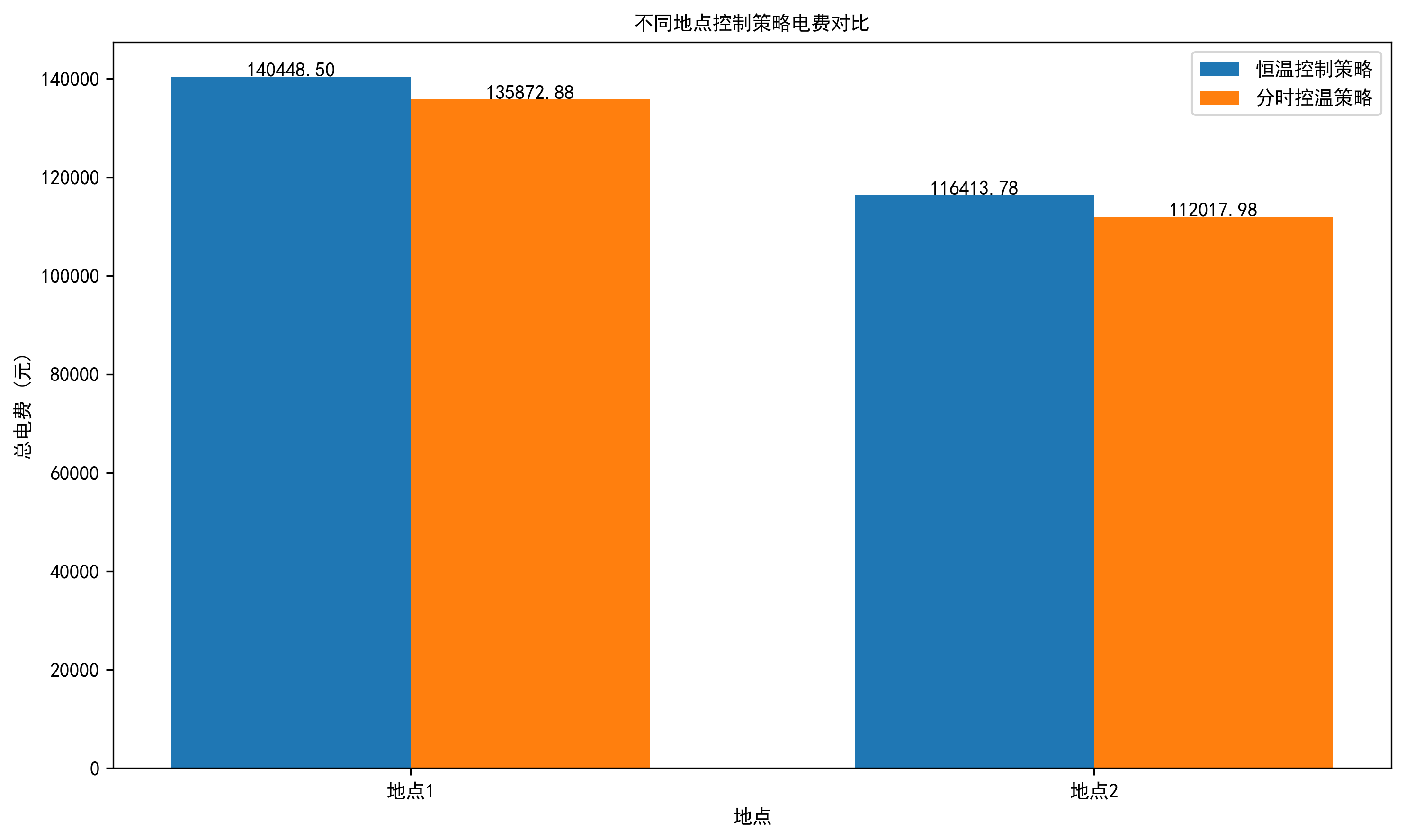
需要更多内容请关注!全文免费分享!
2.代码
import pandas as pd
import numpy as np
import matplotlib.pyplot as plt
import os
import glob
from matplotlib.font_manager import FontProperties
from scipy.optimize import minimize
import datetime
import warnings
warnings.filterwarnings('ignore')

# 设置中文字体
try:
    font = FontProperties(fname=r"C:\Windows\Fonts\simhei.ttf")
    plt.rcParams['font.sans-serif'] = ['SimHei']
    plt.rcParams['axes.unicode_minus'] = False
except:
    font = FontProperties()

# 数据路径
base_path = r"5.15长三角数学建模\2025年第五届长三角高校数学建模竞赛赛题\2025年第五届长三角高校数学建模竞赛赛题\2025长三角赛题B:空气源热泵供暖的温度预测"
location1_heating_path = os.path.join(base_path, "附件2", "地点1", "供热历史数据")
location2_heating_path = os.path.join(base_path, "附件2", "地点2", "供热历史数据")

# 电价设置
day_price = 1.2  # 日间电价 (元/度)
night_price = 0.6  # 夜间电价 (元/度)

def read_heating_data(folder_path):
    """读取供热历史数据"""
    all_data = []

    # 获取所有Excel文件
    files = glob.glob(os.path.join(folder_path, "*.xlsx"))

    for file in files:
        try:
            # 从文件名中提取年份信息
            filename = os.path.basename(file)
            year = filename.split('_')[1][:4]

            # 读取Excel文件
            df = pd.read_excel(file)

            # 添加年份信息
            df['年份'] = year

            # 重命名环境温度列
            if '环境温度(℃)' in df.columns:
                df = df.rename(columns={'环境温度(℃)': '室外温度'})

            # 重命名供水和回水温度列
            if '供温(℃)' in df.columns:
                df = df.rename(columns={'供温(℃)': '供水温度'})
            if '回温(℃)' in df.columns:
                df = df.rename(columns={'回温(℃)': '回水温度'})

            # 重命名功率列
            if '热泵功率(kw)' in df.columns:
                df = df.rename(columns={'热泵功率(kw)': '功率'})

            all_data.append(df)
        except Exception as e:
            print(f"读取文件 {file} 时出错: {e}")

    # 合并所有数据
    if all_data:
        combined_data = pd.concat(all_data, ignore_index=True)
        return combined_data
    else:
        return pd.DataFrame()

def preprocess_data(df):
    """数据预处理"""
    # 确保时间列是datetime类型
    if '时间' in df.columns:
        df['时间'] = pd.to_datetime(df['时间'])

        # 提取时间特征
        df['小时'] = df['时间'].dt.hour
        df['日期'] = df['时间'].dt.date
        df['月份'] = df['时间'].dt.month
        df['星期'] = df['时间'].dt.dayofweek

        # 判断是否为夜间(22:00-6:00)
        df['是否夜间'] = ((df['小时'] >= 22) | (df['小时'] < 6)).astype(int)

        # 添加电价列
        df['电价'] = df['是否夜间'].apply(lambda x: night_price if x == 1 else day_price)

    # 处理缺失值
    for col in ['室外温度', '供水温度', '回水温度', '功率']:
        if col in df.columns:
            df[col] = df[col].interpolate(method='linear')

    return df

def thermal_model(params, T_in_init, T_out, Q_heat, dt=3600):
    """
    建筑热力学模型

    参数:
    params: [C, U] - C是热容量,U是传热系数
    T_in_init: 初始室内温度
    T_out: 室外温度序列
    Q_heat: 热泵提供的热量序列
    dt: 时间步长(秒),默认为1小时

    返回:
    T_in: 预测的室内温度序列
    """
    C, U = params
    n = len(T_out)
    T_in = np.zeros(n)
    T_in[0] = T_in_init

    for i in range(1, n):
        dT = dt/C * (Q_heat[i-1] - U * (T_in[i-1] - T_out[i-1]))
        T_in[i] = T_in[i-1] + dT

    return T_in

def estimate_power_from_temp_diff(temp_diff, base_power=5000, factor=500):
    """根据温差估算所需功率"""
    return base_power + factor * temp_diff

def calculate_electricity_cost(power_kw, hours, price_per_kwh):
    """计算电费"""
    return power_kw * hours * price_per_kwh

def constant_temperature_control(df, target_temp=20.0, C=1e6, U=1000):
    """
    恒温控制策略:保持室内温度恒定在目标温度

    参数:
    df: 包含室外温度数据的DataFrame
    target_temp: 目标室内温度,默认20℃
    C: 建筑热容量
    U: 传热系数

    返回:
    result_df: 包含控制结果的DataFrame
    """
    result = []

    # 按日期分组处理
    for date, day_data in df.groupby('日期'):
        day_data = day_data.sort_values('小时')

        for _, row in day_data.iterrows():
            hour = row['小时']
            outdoor_temp = row['室外温度']
            is_night = row['是否夜间']
            price = row['电价']

            # 计算维持目标温度所需的热量
            temp_diff = target_temp - outdoor_temp
            required_power = estimate_power_from_temp_diff(temp_diff)

            # 计算电费
            electricity_cost = calculate_electricity_cost(required_power/1000, 1, price)

            result.append({
                '日期': date,
                '小时': hour,
                '室外温度': outdoor_temp,
                '目标室内温度': target_temp,
                '实际室内温度': target_temp,
                '是否夜间': is_night,
                '电价': price,
                '功率': required_power,
                '电费': electricity_cost
            })

    return pd.DataFrame(result)

def optimize_temperature_settings(df, C=1e6, U=1000, comfort_min=19.0, comfort_max=21.0):
    """
    分时控温策略:优化每个时间点的温度设定,最小化电费

    参数:
    df: 包含室外温度数据的DataFrame
    C: 建筑热容量
    U: 传热系数
    comfort_min: 舒适温度下限
    comfort_max: 舒适温度上限

    返回:
    result_df: 包含优化结果的DataFrame
    """
    result = []

    # 按日期分组处理
    for date, day_data in df.groupby('日期'):
        day_data = day_data.sort_values('小时')

        # 确保每天有24小时的数据
        hours_in_day = day_data['小时'].unique()
        if len(hours_in_day) < 24:
            print(f"警告: {date}日数据不足24小时,跳过该日期")
            continue

        hours = day_data['小时'].values
        outdoor_temps = day_data['室外温度'].values

        # 创建24小时的夜间标志和电价数组
        is_night = np.zeros(24)
        prices = np.zeros(24)

        # 填充夜间标志和电价数组
        for i in range(24):
            is_night[i] = 1 if (i >= 22 or i < 6) else 0
            prices[i] = night_price if is_night[i] == 1 else day_price

        # 确保室外温度数组长度为24
        if len(outdoor_temps) != 24:
            # 如果数据不足24小时,使用插值填充
            hour_indices = np.array(hours)
            full_hours = np.arange(24)
            outdoor_temps_full = np.interp(full_hours, hour_indices, outdoor_temps)
            outdoor_temps = outdoor_temps_full

        # 初始化温度和功率
        indoor_temps = np.ones(24) * 20.0  # 初始全天设为20℃
        powers = np.zeros(24)

        # 优化函数:最小化电费
        def objective(temps):
            total_cost = 0
            curr_temps = np.copy(temps)

            # 模拟24小时温度变化和能耗
            for i in range(24):
                # 计算当前小时所需功率
                temp_diff = curr_temps[i] - outdoor_temps[i]
                power = estimate_power_from_temp_diff(temp_diff)
                powers[i] = power

                # 计算电费
                cost = calculate_electricity_cost(power/1000, 1, prices[i])
                total_cost += cost

                # 更新后续4小时的温度(热惯性影响)
                if i < 20:  # 避免索引越界
                    decay_factor = 0.8  # 温度衰减因子
                    for j in range(1, 5):
                        if i+j < 24:
                            # 温度会逐渐衰减到室外温度
                            natural_decay = (curr_temps[i] - outdoor_temps[i+j]) * (decay_factor ** j)
                            curr_temps[i+j] = max(outdoor_temps[i+j] + natural_decay, curr_temps[i+j])

            return total_cost

        # 约束条件:温度在舒适区间内
        def constraint(temps):
            return np.all((temps >= comfort_min) & (temps <= comfort_max))

        # 初始猜测:夜间温度略高,白天温度略低
        initial_guess = np.ones(24) * 20.0
        for i in range(24):
            if is_night[i] == 1:
                initial_guess[i] = 20.8  # 夜间温度略高
            else:
                initial_guess[i] = 19.5  # 白天温度略低

        # 优化求解
        bounds = [(comfort_min, comfort_max) for _ in range(24)]

        # 使用模拟退火算法进行优化
        def simulated_annealing():
            current_solution = initial_guess
            current_cost = objective(current_solution)
            best_solution = current_solution
            best_cost = current_cost
            temperature = 1.0
            cooling_rate = 0.95

            for iteration in range(1000):
                # 生成新解
                new_solution = current_solution + np.random.normal(0, 0.3, 24)
                new_solution = np.clip(new_solution, comfort_min, comfort_max)

                # 计算新解的成本
                new_cost = objective(new_solution)

                # 决定是否接受新解
                if new_cost < current_cost or np.random.random() < np.exp((current_cost - new_cost) / temperature):
                    current_solution = new_solution
                    current_cost = new_cost

                # 更新最优解
                if new_cost < best_cost:
                    best_solution = new_solution
                    best_cost = new_cost

                # 降低温度
                temperature *= cooling_rate

            return best_solution

        # 执行优化
        optimal_temps = simulated_annealing()

        # 重新计算最优解对应的功率和成本
        for i in range(24):
            temp_diff = optimal_temps[i] - outdoor_temps[i]
            power = estimate_power_from_temp_diff(temp_diff)
            cost = calculate_electricity_cost(power/1000, 1, prices[i])

            result.append({
                '日期': date,
                '小时': i,
                '室外温度': outdoor_temps[i],
                '目标室内温度': optimal_temps[i],
                '实际室内温度': optimal_temps[i],  # 简化模型,假设实际温度等于目标温度
                '是否夜间': is_night[i],
                '电价': prices[i],
                '功率': power,
                '电费': cost
            })

    return pd.DataFrame(result)

def compare_strategies(constant_df, optimized_df, location_name):
    """比较两种控制策略的效果"""
    # 计算总电费和平均功率
    constant_total_cost = constant_df['电费'].sum()
    optimized_total_cost = optimized_df['电费'].sum()
    constant_avg_power = constant_df['功率'].mean()
    optimized_avg_power = optimized_df['功率'].mean()

    cost_saving = constant_total_cost - optimized_total_cost
    cost_saving_percent = (cost_saving / constant_total_cost) * 100

    print(f"\n{location_name}控制策略对比:")
    print(f"恒温控制策略总电费: {constant_total_cost:.2f}元")
    print(f"分时控温策略总电费: {optimized_total_cost:.2f}元")
    print(f"节省电费: {cost_saving:.2f}元 ({cost_saving_percent:.2f}%)")
    print(f"恒温控制策略平均功率: {constant_avg_power:.2f}W")
    print(f"分时控温策略平均功率: {optimized_avg_power:.2f}W")

    # 创建图表
    fig, axes = plt.subplots(3, 1, figsize=(12, 15))

    # 选择一天的数据进行可视化
    sample_date = constant_df['日期'].unique()[0]
    constant_day = constant_df[constant_df['日期'] == sample_date]
    optimized_day = optimized_df[optimized_df['日期'] == sample_date]

    # 确保两个数据集都有相同的小时数据
    constant_day = constant_day.sort_values('小时')
    optimized_day = optimized_day.sort_values('小时')

    # 1. 室内温度对比
    axes[0].plot(constant_day['小时'], constant_day['实际室内温度'], 'b-', marker='o', label='恒温控制')
    axes[0].plot(optimized_day['小时'], optimized_day['实际室内温度'], 'r-', marker='s', label='分时控温')
    axes[0].plot(optimized_day['小时'], optimized_day['室外温度'], 'g-', marker='^', label='室外温度')
    axes[0].axhspan(19, 21, alpha=0.2, color='green', label='舒适区间')
    axes[0].set_title(f'{location_name}室内温度对比', fontproperties=font)
    axes[0].set_xlabel('小时', fontproperties=font)
    axes[0].set_ylabel('温度 (°C)', fontproperties=font)
    axes[0].set_xticks(range(0, 24))
    axes[0].legend(prop=font)
    axes[0].grid(True)

    # 标记夜间区域
    for i in range(24):
        if i >= 22 or i < 6:
            axes[0].axvspan(i-0.5, i+0.5, alpha=0.1, color='blue')

    # 2. 功率对比
    axes[1].plot(constant_day['小时'], constant_day['功率'], 'b-', marker='o', label='恒温控制')
    axes[1].plot(optimized_day['小时'], optimized_day['功率'], 'r-', marker='s', label='分时控温')
    axes[1].set_title(f'{location_name}功率对比', fontproperties=font)
    axes[1].set_xlabel('小时', fontproperties=font)
    axes[1].set_ylabel('功率 (W)', fontproperties=font)
    axes[1].set_xticks(range(0, 24))
    axes[1].legend(prop=font)
    axes[1].grid(True)

    # 标记夜间区域
    for i in range(24):
        if i >= 22 or i < 6:
            axes[1].axvspan(i-0.5, i+0.5, alpha=0.1, color='blue')

    # 3. 电费对比
    axes[2].plot(constant_day['小时'], constant_day['电费'], 'b-', marker='o', label='恒温控制')
    axes[2].plot(optimized_day['小时'], optimized_day['电费'], 'r-', marker='s', label='分时控温')
    axes[2].set_title(f'{location_name}电费对比', fontproperties=font)
    axes[2].set_xlabel('小时', fontproperties=font)
    axes[2].set_ylabel('电费 (元)', fontproperties=font)
    axes[2].set_xticks(range(0, 24))
    axes[2].legend(prop=font)
    axes[2].grid(True)

    # 标记夜间区域
    for i in range(24):
        if i >= 22 or i < 6:
            axes[2].axvspan(i-0.5, i+0.5, alpha=0.1, color='blue')

    plt.tight_layout()
    plt.savefig(f'{location_name}_控制策略对比.png', dpi=300, bbox_inches='tight')

    # 保存结果到CSV
    constant_df.to_csv(f'{location_name}_恒温控制策略.csv', index=False, encoding='utf-8-sig')
    optimized_df.to_csv(f'{location_name}_分时控温策略.csv', index=False, encoding='utf-8-sig')

    return {
        'constant_total_cost': constant_total_cost,
        'optimized_total_cost': optimized_total_cost,
        'cost_saving': cost_saving,
        'cost_saving_percent': cost_saving_percent,
        'constant_avg_power': constant_avg_power,
        'optimized_avg_power': optimized_avg_power
    }

def main():
    """主函数"""
    print("开始分析空气源热泵供暖的温度控制优化问题...")

    # 读取地点1数据
    print("\n读取地点1数据...")
    location1_data = read_heating_data(location1_heating_path)

    if not location1_data.empty:
        print(f"成功读取地点1数据,共{len(location1_data)}条记录")

        # 数据预处理
        location1_data = preprocess_data(location1_data)

        # 恒温控制策略
        print("\n计算地点1恒温控制策略...")
        constant_control1 = constant_temperature_control(location1_data)

        # 分时控温策略
        print("\n计算地点1分时控温策略...")
        optimized_control1 = optimize_temperature_settings(location1_data)

        # 比较两种策略
        compare_results1 = compare_strategies(constant_control1, optimized_control1, "地点1")
    else:
        print("未能读取地点1数据")

    # 读取地点2数据
    print("\n读取地点2数据...")
    location2_data = read_heating_data(location2_heating_path)

    if not location2_data.empty:
        print(f"成功读取地点2数据,共{len(location2_data)}条记录")

        # 数据预处理
        location2_data = preprocess_data(location2_data)

        # 恒温控制策略
        print("\n计算地点2恒温控制策略...")
        constant_control2 = constant_temperature_control(location2_data)

        # 分时控温策略
        print("\n计算地点2分时控温策略...")
        optimized_control2 = optimize_temperature_settings(location2_data)

        # 比较两种策略
        compare_results2 = compare_strategies(constant_control2, optimized_control2, "地点2")
    else:
        print("未能读取地点2数据")

    # 综合分析
    if 'compare_results1' in locals() and 'compare_results2' in locals():
        print("\n综合分析:")
        avg_saving_percent = (compare_results1['cost_saving_percent'] + compare_results2['cost_saving_percent']) / 2
        print(f"平均节省电费比例: {avg_saving_percent:.2f}%")

        # 创建综合对比图表
        plt.figure(figsize=(10, 6))

        locations = ['地点1', '地点2']
        constant_costs = [compare_results1['constant_total_cost'], compare_results2['constant_total_cost']]
        optimized_costs = [compare_results1['optimized_total_cost'], compare_results2['optimized_total_cost']]

        x = np.arange(len(locations))
        width = 0.35

        plt.bar(x - width/2, constant_costs, width, label='恒温控制策略')
        plt.bar(x + width/2, optimized_costs, width, label='分时控温策略')

        plt.title('不同地点控制策略电费对比', fontproperties=font)
        plt.xlabel('地点', fontproperties=font)
        plt.ylabel('总电费 (元)', fontproperties=font)
        plt.xticks(x, locations)
        plt.legend(prop=font)

        for i, v in enumerate(constant_costs):
            plt.text(i - width/2, v + 0.5, f'{v:.2f}', ha='center', fontproperties=font)

        for i, v in enumerate(optimized_costs):
            plt.text(i + width/2, v + 0.5, f'{v:.2f}', ha='center', fontproperties=font)

        plt.tight_layout()
        plt.savefig('综合电费对比.png', dpi=300, bbox_inches='tight')

    print("\n分析完成!")

if __name__ == "__main__":
main()获取方式( 企鹅号:746874232)


GitCode 天启AI是一款由 GitCode 团队打造的智能助手,基于先进的LLM(大语言模型)与多智能体 Agent 技术构建,致力于为用户提供高效、智能、多模态的创作与开发支持。它不仅支持自然语言对话,还具备处理文件、生成 PPT、撰写分析报告、开发 Web 应用等多项能力,真正做到“一句话,让 Al帮你完成复杂任务”。
更多推荐


 10
10 0
0- 0


 已为社区贡献5条内容

所有评论(0)