提示：文章写完后，目录可以自动生成，如何生成可参考右边的帮助文档

---

前言

笔者权当做笔记，借鉴的是《Python 深度学习》这本书，里面的代码也都是书上的代码，用的是jupyter notebook 编写代码

---

提示：以下是本篇文章正文内容，下面案例可供参考

一、路透社数据集

包含了许多短新闻及其对应的主题。是一个简单广泛的文本分类数据集。包括46个不同的主题：某些主题的样本更多，训练集中每个主题都有至少10个样本。
和IMDB一样，路透社数据集也是内置在Keras的一部分

二、步骤

1.导入Keras

---

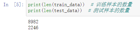
2、加载路透社数据集

from keras.datasets import reuters

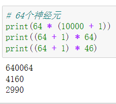
# num_words=10 000 限制的是前10 000个最常出现的单词
(train_data, train_labels), (test_data, test_labels) = reuters.load_data(num_words=10000)

我们有8982个训练样本和2246个测试样本

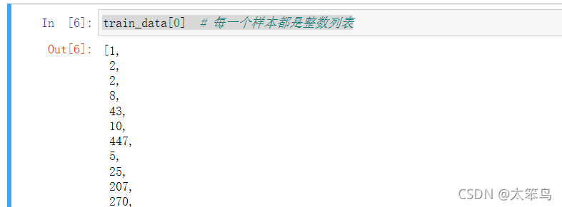
train_data[0]  # 每一个样本都是整数列表

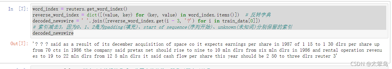
# 将索引解码为单词
word_index = reuters.get_word_index()
reverse_word_index = dict([(value, key) for (key, value) in word_index.items()])  # 反转字典
decoded_newswire = ' '.join([reverse_word_index.get(i - 3, '?') for i in train_data[0]])
# 索引减去3，因为0、1、2是为padding(填充)、start of sequence(序列开始)、unknown(未知词)分别保留的索引
decoded_newswire

3、准备数据

和上一次一样，要将数据向量化
同样我们还用one-hot编码

import numpy as np

def vectorize_sequences(sequences, dimension=10000):
    results = np.zeros((len(sequences), dimension))  # (8982, 10000)的零矩阵
    for i, sequence in enumerate(sequences):  # enumerate 这个就是从0开始编码的那种
        results[i, sequence] = 1.
    return results


# 数据向量化
x_train = vectorize_sequences(train_data)
x_test = vectorize_sequences(test_data)

def to_one_hot(labels, dimension=46):
    results = np.zeros((len(labels), dimension))  # (8982, 46)的零矩阵
    for i, label in enumerate(labels):
        results[i, label] = 1.  # 相当于就是在编号i这一行，然后对应的类别号列编成1
    return results

# 标签向量化
one_hot_train_labels = to_one_hot(train_labels)
one_hot_test_labels = to_one_hot(test_labels)

上面的那个也可以用Keras内置方法实现这个操作

# 上述向量化其实Keras内置也可以实现
from keras.utils.np_utils import to_categorical
# 独热编码
one_hot_train_labels = to_categorical(train_labels)
one_hot_test_labels = to_categorical(test_labels)

4、构建网络

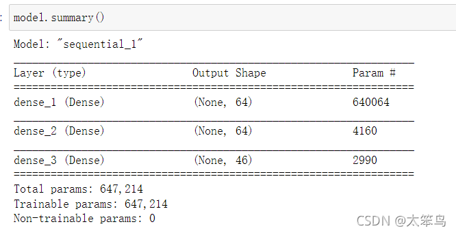
4.1 构建模型

from keras import models
from keras import layers

model = models.Sequential()

model.add(layers.Dense(64, activation='relu', input_shape=(10000, )))
model.add(layers.Dense(64, activation='relu'))
model.add(layers.Dense(46, activation='softmax'))

4.2 编译模型

# 多元分类的交叉熵 loss='categorical_crossentropy'
model.compile(optimizer='rmsprop', loss='categorical_crossentropy', metrics=['accuracy'])

4.3 准备验证集

# 和上次的一样用切片来做即可
x_val = x_train[:1000]  # 前1000个是验证集
partial_x_train = x_train[1000:]

y_val = one_hot_train_labels[:1000]
partial_y_train = one_hot_train_labels[1000:]

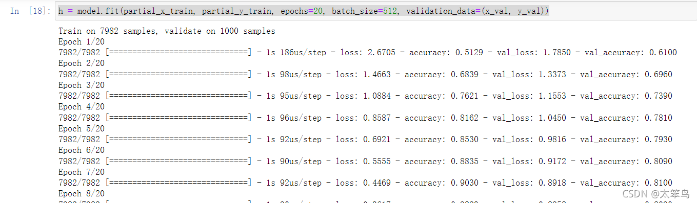
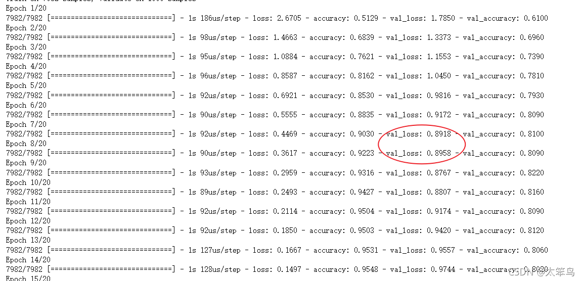
4.4 训练模型

h = model.fit(partial_x_train, partial_y_train, epochs=20, batch_size=512, validation_data=(x_val, y_val))

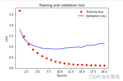
5、绘制图像

import matplotlib.pyplot as plt

loss = h.history['loss']
val_loss = h.history['val_loss']

epochs = range(1, len(loss) + 1)

plt.plot(epochs, loss, 'ro', label='Training loss')
plt.plot(epochs, val_loss, 'b', label='Validation loss')
plt.title('Training and validation loss')
plt.xlabel('Epochs')
plt.ylabel('Loss')
plt.legend()
plt.show()

plt.clf()  # 清空图像

acc = h.history['accuracy']
val_acc = h.history['val_accuracy']

plt.plot(epochs, acc, 'ro', label='Training acc')
plt.plot(epochs, val_acc, 'b', label='Validation acc')
plt.title('Training and validation accuracy')
plt.xlabel('Epochs')
plt.ylabel('Accuracy')
plt.legend()
plt.show()

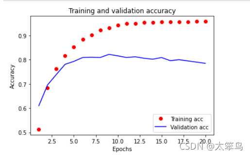
我们得出在第7轮的之后要出现“过拟合”现象

6、重新训练一个新的模型

model = models.Sequential()
model.add(layers.Dense(64, activation='relu', input_shape=(10000, )))
model.add(layers.Dense(64, activation='relu'))
model.add(layers.Dense(46, activation='softmax'))

model.compile(optimizer='rmsprop', loss='categorical_crossentropy', metrics=['accuracy'])
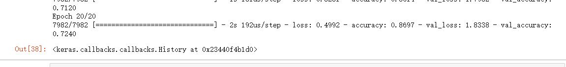
model.fit(partial_x_train, partial_y_train, epochs=7, batch_size=512, validation_data=(x_val, y_val))
results = model.evaluate(x_test, one_hot_test_labels)

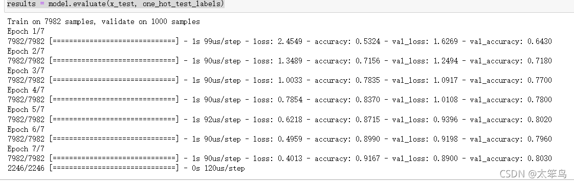
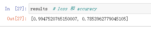
只能得到约78%的精度

import copy  # 复制

test_labels_copy = copy.copy(test_labels)
np.random.shuffle(test_labels_copy)
hits_array = np.array(test_labels) == np.array(test_labels_copy)
float(np.sum(hits_array)) / len(test_labels)

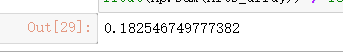
完全随机的精度是18%

7、使用训练好的网络在新数据上生成预测结果

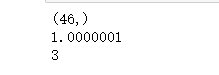
predictions = model.predict(x_test)
print(predictions[0].shape)
print(str(np.sum(predictions[0])))  # 概率加起来就是1
print(np.argmax(predictions[0]))  # 这个数据哪一个分类概率最大 

8、处理标签和损失的另一种方法

就是使用loss="sparse_categotical_crossentropy"这样Keras会自动进行分类编码

9、 中间层维度足够大的重要性

model = models.Sequential()
model.add(layers.Dense(64, activation='relu', input_shape=(10000, )))
model.add(layers.Dense(4, activation='relu'))  # 测试中间层维度变小带来的影响
model.add(layers.Dense(46, activation='softmax'))

model.compile(optimizer='rmsprop', loss='categorical_crossentropy', metrics=['accuracy'])

model.fit(partial_x_train, partial_y_train, epochs=20, batch_size=128, validation_data=(x_val, y_val))

可以很清楚的发现，中间层压缩到很小的维度后，准确率变低了许多，可能的原因是信息的缺失。

---

总结

这个是我单纯看书跟着敲的，权当作笔记了，后续还要继续学习。强推《Python 深度学习》🙂