说明：研究了绘制这个脑的轮廓图需要哪些函数，一些问题和bug，三维的通道应该使用什么投影方式，一个可用的基本绘图代码。

我们可以使用eeglab或者mne的函数绘制一个脑区带各种的如热力图，或者通道的psd，以及project图。
如何绘制一个空的图，并且自己可以进行一些diy。

我们可以知道有许多类似于下面这个函数的调用方式。

plot_topo()

在mne中，我们可以找到这个函数，是如何绘制一个二维的头的轮廓的。

from mne.viz.topomap import _make_head_outlines

此处给出函数的定义，可以看到，这个是按照给定的参数，返回的默认绘制的一些点。

mne源码

def _make_head_outlines(sphere, pos, outlines, clip_origin):
    """Check or create outlines for topoplot."""
    assert isinstance(sphere, np.ndarray)
    x, y, _, radius = sphere
    del sphere

    if outlines in ("head", None):
        ll = np.linspace(0, 2 * np.pi, 101)
        head_x = np.cos(ll) * radius + x
        head_y = np.sin(ll) * radius + y
        dx = np.exp(np.arccos(np.deg2rad(12)) * 1j)
        dx, dy = dx.real, dx.imag
        nose_x = np.array([-dx, 0, dx]) * radius + x
        nose_y = np.array([dy, 1.15, dy]) * radius + y
        ear_x = np.array(
            [0.497, 0.510, 0.518, 0.5299, 0.5419, 0.54, 0.547, 0.532, 0.510, 0.489]
        ) * (radius * 2)
        ear_y = (
            np.array(
                [
                    0.0555,
                    0.0775,
                    0.0783,
                    0.0746,
                    0.0555,
                    -0.0055,
                    -0.0932,
                    -0.1313,
                    -0.1384,
                    -0.1199,
                ]
            )
            * (radius * 2)
            + y
        )

        if outlines is not None:
            # Define the outline of the head, ears and nose
            outlines_dict = dict(
                head=(head_x, head_y),
                nose=(nose_x, nose_y),
                ear_left=(-ear_x + x, ear_y),
                ear_right=(ear_x + x, ear_y),
            )
        else:
            outlines_dict = dict()

        # Make the figure encompass slightly more than all points
        # We probably want to ensure it always contains our most
        # extremely positioned channels, so we do:
        mask_scale = max(1.0, np.linalg.norm(pos, axis=1).max() * 1.01 / radius)
        outlines_dict["mask_pos"] = (mask_scale * head_x, mask_scale * head_y)
        clip_radius = radius * mask_scale
        outlines_dict["clip_radius"] = (clip_radius,) * 2
        outlines_dict["clip_origin"] = clip_origin
        outlines = outlines_dict

    elif isinstance(outlines, dict):
        if "mask_pos" not in outlines:
            raise ValueError("You must specify the coordinates of the image mask.")
    else:
        raise ValueError("Invalid value for `outlines`.")

    return outlines


def _draw_outlines(ax, outlines):
    """Draw the outlines for a topomap."""
    from matplotlib import rcParams

    outlines_ = {k: v for k, v in outlines.items() if k not in ["patch"]}
    for key, (x_coord, y_coord) in outlines_.items():
        if "mask" in key or key in ("clip_radius", "clip_origin"):
            continue
        ax.plot(
            x_coord,
            y_coord,
            color=rcParams["axes.edgecolor"],
            linewidth=1,
            clip_on=False,
        )
    return outlines_

ai解析

以下是对该函数的详细分析，包括其功能、实现逻辑、参数和返回值。

---

函数功能

_make_head_outlines 用于生成或验证拓扑图（topoplot）中头部轮廓的几何信息。它根据输入的球体参数和电极位置，生成头部外圆、鼻子、耳朵等轮廓，并支持自定义裁剪区域。

---

参数说明

1. sphere

   • 类型：np.ndarray，形状为 (4,)。
   • 描述：头部球体模型的参数，格式为 (x, y, z, radius)，其中 (x, y, z) 是球心坐标，radius 是球体半径。

2. pos

   • 类型：np.ndarray，形状为 (n_channels, 2)。
   • 描述：电极或传感器在 2D 平面上的投影坐标。

3. outlines

   • 类型：str 或 dict 或 None。
   • 描述：指定头部轮廓的生成方式或直接提供轮廓字典。
     • "head"：生成默认的头部轮廓（包括头部外圆、鼻子和耳朵）。
     • None：不生成任何轮廓。
     • dict：直接使用传入的轮廓字典（需包含 "mask_pos" 键）。

4. clip_origin

   • 类型：tuple，形状为 (2,)。
   • 描述：裁剪区域的参考点坐标，用于定义裁剪区域的中心。

---

返回值

返回一个字典 outlines_dict，包含以下键值对：

• head：头部外圆的坐标，形状为 (2, 101)，表示 101 个点的 (x, y) 坐标。
• nose：鼻子轮廓的坐标，形状为 (2, 3)，表示 3 个点的 (x, y) 坐标。
• ear_left：左耳轮廓的坐标，形状为 (2, 10)，表示 10 个点的 (x, y) 坐标。
• ear_right：右耳轮廓的坐标，形状为 (2, 10)，表示 10 个点的 (x, y) 坐标。
• mask_pos：用于定义图像掩模的放大头部轮廓，形状为 (2, 101)。
• clip_radius：裁剪区域的半径，形状为 (2,)。
• clip_origin：裁剪区域的参考点坐标，形状为 (2,)。

---

实现逻辑

1. 验证输入参数

   • 检查 sphere 是否为 np.ndarray。
   • 提取球心坐标 (x, y) 和半径 radius。

2. 生成默认头部轮廓

   • 如果 outlines 为 "head" 或 None，生成以下轮廓：
     • 头部外圆：使用 101 个点生成一个圆形。
     • 鼻子：基于预定义的几何形状生成 3 个点。
     • 鼻子长度由 radius 决定。
     • 鼻子角度为 12°。
     • 使用复数运算计算鼻子点的坐标。
     • 耳朵：基于预定义的几何形状生成 10 个点。
     • 左耳和右耳对称生成。
   • 如果 outlines 为 None，则仅生成 mask_pos 和裁剪区域信息。

3. 计算掩模和裁剪区域

   • mask_pos：根据电极位置的最大距离，放大头部外圆以确保所有电极点被包含。
   • clip_radius：根据 mask_scale 计算裁剪区域的半径。
   • clip_origin：直接使用传入的裁剪参考点。

4. 验证自定义轮廓字典

   • 如果 outlines 是字典，检查是否包含 "mask_pos" 键。

5. 返回轮廓字典

   • 返回生成的或验证后的轮廓字典。

---

代码逐行解析

def _make_head_outlines(sphere, pos, outlines, clip_origin):
    """Check or create outlines for topoplot."""
    assert isinstance(sphere, np.ndarray)  # 确保 sphere 是 np.ndarray
    x, y, _, radius = sphere  # 提取球心坐标和半径
    del sphere  # 删除 sphere 以节省内存

    if outlines in ("head", None):  # 如果 outlines 是 "head" 或 None
        ll = np.linspace(0, 2 * np.pi, 101)  # 生成 101 个角度值
        head_x = np.cos(ll) * radius + x  # 计算头部外圆的 x 坐标
        head_y = np.sin(ll) * radius + y  # 计算头部外圆的 y 坐标

        # 计算鼻子点的坐标
        dx = np.exp(np.arccos(np.deg2rad(12)) * 1j)  # 使用复数运算计算鼻子点的偏移
        dx, dy = dx.real, dx.imag  # 提取实部和虚部
        nose_x = np.array([-dx, 0, dx]) * radius + x  # 鼻子点的 x 坐标
        nose_y = np.array([dy, 1.15, dy]) * radius + y  # 鼻子点的 y 坐标

        # 计算耳朵点的坐标
        ear_x = np.array([0.497, 0.510, ..., 0.489]) * (radius * 2)  # 左耳 x 坐标
        ear_y = np.array([0.0555, 0.0775, ..., -0.1199]) * (radius * 2) + y  # 左耳 y 坐标

        if outlines is not None:  # 如果 outlines 是 "head"
            # 定义头部、鼻子和耳朵的轮廓
            outlines_dict = dict(
                head=(head_x, head_y),
                nose=(nose_x, nose_y),
                ear_left=(-ear_x + x, ear_y),  # 左耳
                ear_right=(ear_x + x, ear_y),  # 右耳
            )
        else:  # 如果 outlines 是 None
            outlines_dict = dict()  # 空字典

        # 计算掩模区域,确定插值算法的有效区域
        mask_scale = max(1.0, np.linalg.norm(pos, axis=1).max() * 1.01 / radius)
        outlines_dict["mask_pos"] = (mask_scale * head_x, mask_scale * head_y)
        clip_radius = radius * mask_scale
        outlines_dict["clip_radius"] = (clip_radius,) * 2
        outlines_dict["clip_origin"] = clip_origin
        outlines = outlines_dict

    elif isinstance(outlines, dict):  # 如果 outlines 是字典
        if "mask_pos" not in outlines:  # 检查是否包含 mask_pos
            raise ValueError("You must specify the coordinates of the image mask.")
    else:  # 如果 outlines 是无效值
        raise ValueError("Invalid value for `outlines`.")

    return outlines  # 返回轮廓字典

---

掩模区域的主要作用是：

限制插值范围，确保数据仅在头部轮廓内插值。

裁剪无效区域，使图像仅显示头部内的数据。

支持不同插值模式，增强拓扑图的灵活性和准确性。

总结

• 核心功能：生成或验证拓扑图的头部轮廓。
• 灵活性：支持默认轮廓生成和自定义轮廓输入。
• 应用场景：主要用于 plot_projs_topomap 等拓扑图绘制函数中。

可以绘制一些自定义坐标和布局方式。

使用的方式

默认的参数

#MNE-Python 的默认球体参数为
sphere = np.array([0.0, 0.0, 0.04, 0.095])

这个球体的参数可能根据使用的电极布局的不同而有所区别。

说明

在研究的时候，应该按照大的不同的分类进行区分。

头部半径的实际值会因个体差异而有所不同：

成年人：头部半径通常在 8.5 厘米到 10.5 厘米 之间。（mne默认的参数是9.5cm）

儿童：头部半径较小，通常在 7 厘米到 9 厘米 之间。

如果有MRI的头部扫描数据，可以构建更具体的头部扫描，并拟合球体模型来计算头部的半径。
或者按照电极的位置布局来估计头部的半径。

使用函数

make_sphere_model 用于创建一个球形导体模型（spherical conductor model），主要用于计算脑电（EEG）或脑磁（MEG）的正向解（forward solution）。该模型基于多层球体（如头皮、颅骨、脑脊液和脑组织）的几何和电导率参数。

import numpy as np
from mne import make_sphere_model
info = raw_data.info#raw_data应该是有定位文件和信息的

# 假设 pos 是电极位置的 3D 坐标 (n_channels, 3)
sphere_model = make_sphere_model(r0=(0.0, 0.0, 0.04), head_radius='auto', info=info)
r0 = sphere_model["r0"]  # 球心坐标 (x, y, z)
head_radius = sphere_model["layers"][-1]["rad"] # 头部半径
sphere = np.array([r0[0], r0[1], r0[2], radius])

Fitted sphere radius: 92.9 mm
Origin head coordinates: 1.0 -18.9 7.4 mm
Origin device coordinates: 1.0 -18.9 7.4 mm

Equiv. model fitting -> RV = 0.00348862 %%
mu1 = 0.944723 lambda1 = 0.137154
mu2 = 0.66746 lambda2 = 0.683797
mu3 = -0.267046 lambda3 = -0.0105814
Set up EEG sphere model with scalp radius 92.9 mm

一般采用默认的数据都可以。

手动计算

import numpy as np
from mne import create_info
from mne.channels import make_standard_montage

# 假设 info 是你的数据信息
montage = info.get_montage()

# 获取电极的 3D 坐标
positions = montage.get_positions()
ch_pos = positions['ch_pos']  # 电极名称到坐标的映射
pos = np.array(list(ch_pos.values()))  # 转换为 numpy 数组 (n_channels, 3)
# 计算几何中心
center = np.mean(pos, axis=0)  # (x, y, z)

# 计算每个电极点到几何中心的距离
distances = np.linalg.norm(pos - center, axis=1)

# 计算头部半径（最大距离）
head_radius = np.max(distances)

print(f"头部半径: {head_radius:.4f} 米")

此处计算了一下，头部的半径是0.1108米。

说明此处的pos投影

info = raw_data.info  # 或 epochs.info
montage = info.get_montage()
# pos = np.array([ch['loc'][:2] for ch in info['chs'] if ch['kind'] == 2])  # 提取 EEG 2D 位置
pos_3d = montage.get_positions()['ch_pos']
# 选择 x, y, z 坐标并进行球面投影
def spherical_projection(pos_3d):
    # 提取 x, y, z 坐标
    x = np.array([pos_3d[ch][0] for ch in pos_3d])
    y = np.array([pos_3d[ch][1] for ch in pos_3d])
    z = np.array([pos_3d[ch][2] for ch in pos_3d])

    # 计算距离球心的半径
    r = np.sqrt(x**2 + y**2 + z**2)

    # 球面投影：将 z 坐标映射到一个平面，调整投影系数，避免重叠
    projection_factor = 0.95  # 可以调整此因子来控制投影效果
    x_proj = x / r * projection_factor
    y_proj = y / r * projection_factor

    return np.column_stack((x_proj, y_proj))

pos_2d = spherical_projection(pos_3d)

在实际使用中效果不佳，因为此处的z轴的位置是非零的，在头部偏下的位置的z坐标是负值。
反而会导致x,y的坐标更加接近和重合。
我们可以进行一个简单的修正，如果z是正值，我们保持原来的投影方式不处理（会出现在头皮的上方），如果z是负值，我们进行绝对值的放大。

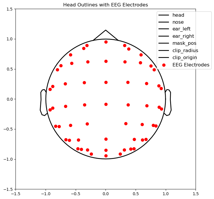
绘制头部轮廓，此处轮廓的坐标放大了10倍，可能是计算单位的原因。
pos的坐标使用直接取x,y的，所以会有些密集

import matplotlib.pyplot as plt
import numpy as np
import mne

# 生成头部轮廓
sphere = np.array([0.0, 0.0, 0.0, 0.1108])  # 适当增大半径

info = raw_data.info  # 或 epochs.info
montage = info.get_montage()
pos = pos_2d
head_outlines = mne.viz.topomap._make_head_outlines(sphere, pos, outlines="head", clip_origin=(0.0, 0.0))

# 创建绘图
fig, ax = plt.subplots(figsize=(8, 8))  # 让图像更清晰
ax.set_aspect("equal")
ax.set_xlim(-1.5, 1.5)
ax.set_ylim(-1.5, 1.5)

# 绘制头部轮廓，此处轮廓放大了10倍，可能是计算单位的原因。
for key, val in head_outlines.items():
    if isinstance(val, (np.ndarray, list, tuple)) :
        if isinstance(val, (list, tuple)):
            val = np.array(val) 
        if val.shape[0] == 2:
            print(f"绘制 {key}:")
            print(val[0], val[1])
            ax.plot(val[0]*10, val[1]*10, color="black", lw=2, label=key)
    else:
        print(f"Unexpected type for {key}: {type(val)}")



# 绘制 EEG 通道（绘制脑电通道的）
ax.scatter(pos[:, 0], pos[:, 1], color="red", s=50, label="EEG Electrodes")

ax.legend(loc='upper right', bbox_to_anchor=(1.1, 1), fontsize=12)

plt.title("Head Outlines with EEG Electrodes")
plt.show()

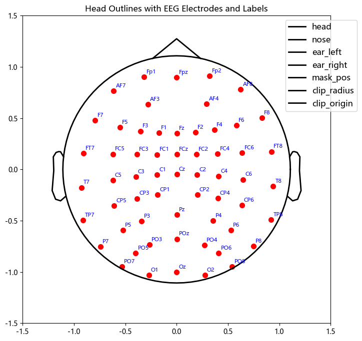
添加绘制通道名称的代码

# 绘制 EEG 通道并添加名称
# 假设 pos 是二维数组（shape: (n_channels, 2)）
# 并且 info.ch_names 是通道名称列表
for i, (x, y) in enumerate(pos):
    # 绘制电极点
    ax.scatter(x , y , color="red", s=50)
    
    # 添加通道名称（注意坐标缩放）
    # 调整偏移量（dx, dy）以避免标签重叠
    ax.annotate(
        text=info.ch_names[i],  # 通道名称
        xy=(x , y ),   # 电极坐标（与 scatter 的坐标一致）
        xytext=(3, 3),         # 标签相对于电极点的偏移量（可调整）
        textcoords="offset points",  # 偏移量单位
        fontsize=8,            # 字体大小
        color="blue",          # 标签颜色
        ha="left",             # 水平对齐方式
        va="bottom"            # 垂直对齐方式
    )

# 添加图例和标题
ax.legend(loc='upper right', bbox_to_anchor=(1.1, 1), fontsize=12)
plt.title("Head Outlines with EEG Electrodes and Labels")
plt.tight_layout()  # 自动调整布局
plt.show()

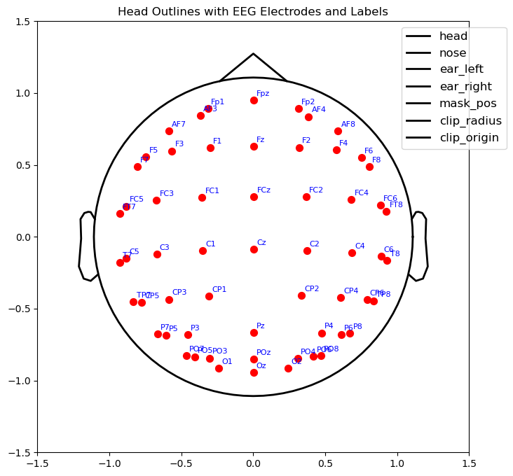
下面我们来讨论一下，有z轴的通道该如何处理，直接舍弃z轴，会导致头下侧的通道重叠。

构造一个坐标映射的函数，从3d坐标到二维平面，感觉可以超过头皮的图像。

#按照设想的来，但是效果不是很好
def custom_projection(pos_3d, k=0.5):
    """
    Args:
        pos_3d: 字典，键为电极名称，值为 (x, y, z) 坐标。
        k: 控制 z<0 时的位移强度（默认0.5）。
    Returns:
        二维坐标数组 (n_channels, 2)
    """
    positions = np.array(list(pos_3d.values()))
    x, y, z = positions[:,0], positions[:,1], positions[:,2]
    r = np.sqrt(x**2 + y**2 + z**2)
    
    # 计算径向单位向量的 x/y 分量
    radial_x = x / r
    radial_y = y / r
    
    # 初始化投影后的坐标
    x_proj = np.copy(x)
    y_proj = np.copy(y)
    
    # 对 z<0 的点进行调整
    mask = z < 0
    delta = -k * z[mask]  # 位移量（因为 z 是负数，所以 -z 是正的）
    x_proj[mask] += delta * radial_x[mask]
    y_proj[mask] += delta * radial_y[mask]
    
    # 归一化到 [-1, 1] 范围（可选）
    scale = 1.0  # 根据需要调整缩放因子
    x_proj /= scale
    y_proj /= scale
    
    return np.column_stack((x_proj, y_proj))

# 使用示例：
pos_2d_custom = custom_projection(pos_3d, k=0.5)

对透视方法的探究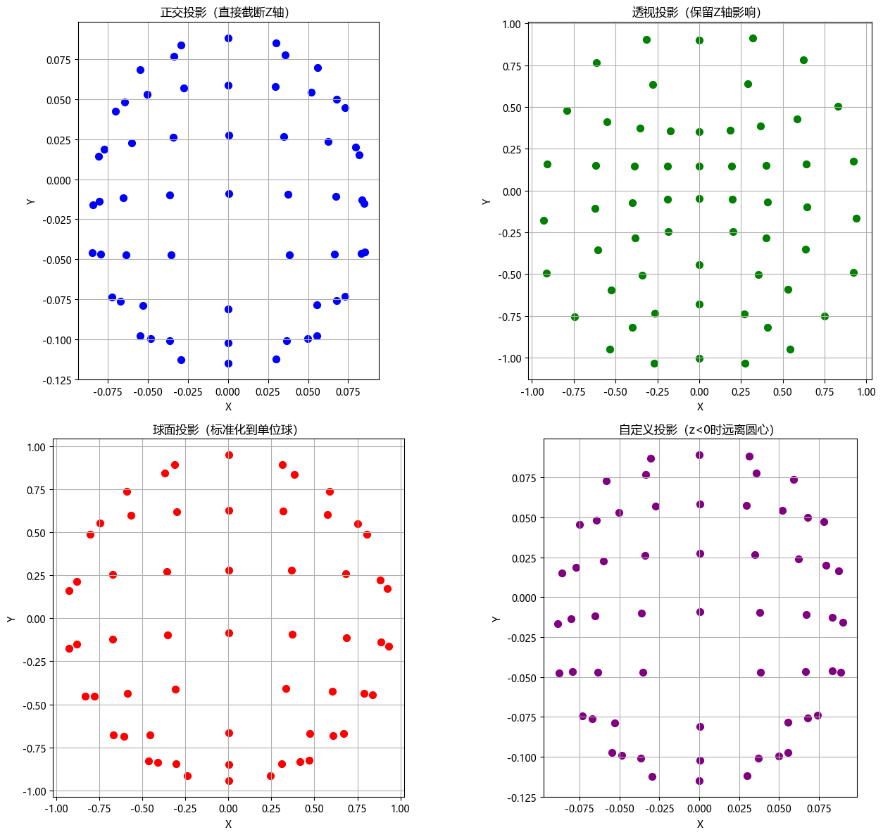

上面绘图的代码
此处省略了导入数据的montage部分。
综上所述，还是

montage = info.get_montage()

import numpy as np
import matplotlib.pyplot as plt
from mne import read_epochs
from matplotlib import rcParams

# # 读取数据
# raw_data = read_epochs("your_data.epochs")  # 替换为实际路径
# montage = raw_data.get_montage()
pos_3d = montage.get_positions()['ch_pos']
rcParams['font.sans-serif'] = ['Microsoft YaHei']  # 使用黑体字体
rcParams['axes.unicode_minus'] = False  # 解决负号显示问题
# 定义所有投影方法
def orthogonal_projection(pos_3d):
    positions = np.array(list(pos_3d.values()))
    return positions[:, :2]

def perspective_projection(pos_3d, epsilon=0.1):
    positions = np.array(list(pos_3d.values()))
    x, y, z = positions[:,0], positions[:,1], positions[:,2]
    x_proj = x / (z + epsilon)
    y_proj = y / (z + epsilon)
    return np.column_stack((x_proj, y_proj))

def spherical_projection(pos_3d):
    positions = np.array(list(pos_3d.values()))
    x, y, z = positions[:,0], positions[:,1], positions[:,2]
    r = np.sqrt(x**2 + y**2 + z**2)
    x_proj = x / r * 0.95
    y_proj = y / r * 0.95
    return np.column_stack((x_proj, y_proj))

def custom_projection(pos_3d, k=0.5):
    positions = np.array(list(pos_3d.values()))
    x, y, z = positions[:,0], positions[:,1], positions[:,2]
    r = np.sqrt(x**2 + y**2 + z**2)
    radial_x = x / r
    radial_y = y / r
    x_proj = np.copy(x)
    y_proj = np.copy(y)
    mask = z < 0
    delta = -k * z[mask]
    x_proj[mask] += delta * radial_x[mask]
    y_proj[mask] += delta * radial_y[mask]
    return np.column_stack((x_proj, y_proj))

# 生成投影结果
pos_ortho = orthogonal_projection(pos_3d)
pos_persp = perspective_projection(pos_3d)
pos_sphere = spherical_projection(pos_3d)
pos_custom = custom_projection(pos_3d, k=0.5)

# 可视化
fig, axes = plt.subplots(2, 2, figsize=(14, 12))

# 正交投影
axes[0,0].scatter(pos_ortho[:,0], pos_ortho[:,1], c='blue', s=50)
axes[0,0].set_title("正交投影（直接截断Z轴）", fontsize=12)
axes[0,0].grid(True)

# 透视投影
axes[0,1].scatter(pos_persp[:,0], pos_persp[:,1], c='green', s=50)
axes[0,1].set_title("透视投影（保留Z轴影响）", fontsize=12)
axes[0,1].grid(True)

# 球面投影
axes[1,0].scatter(pos_sphere[:,0], pos_sphere[:,1], c='red', s=50)
axes[1,0].set_title("球面投影（标准化到单位球）", fontsize=12)
axes[1,0].grid(True)

# 自定义投影
axes[1,1].scatter(pos_custom[:,0], pos_custom[:,1], c='purple', s=50)
axes[1,1].set_title("自定义投影（z<0时远离圆心）", fontsize=12)
axes[1,1].grid(True)

for ax in axes.flat:
    ax.set_xlabel("X", fontsize=10)
    ax.set_ylabel("Y", fontsize=10)
    ax.set_aspect('equal')

plt.tight_layout()
plt.show()

eeglab的标准电极绘制

使用matlab的电极定位的plot2D绘制的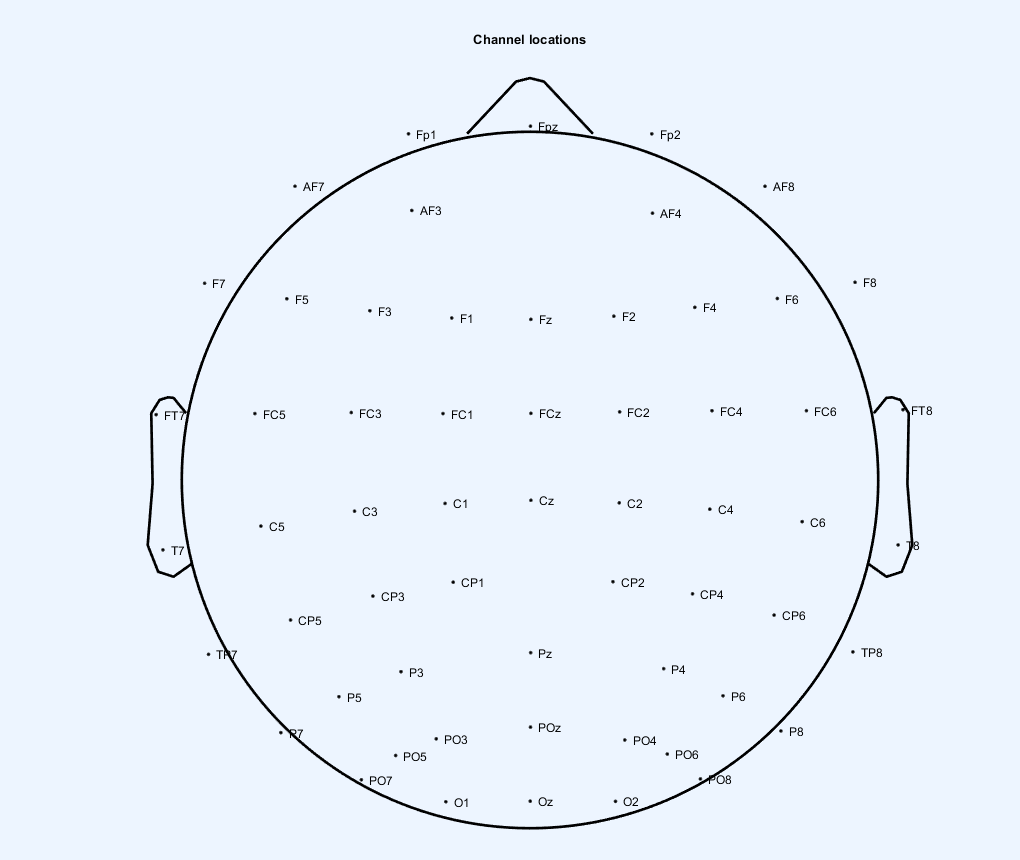


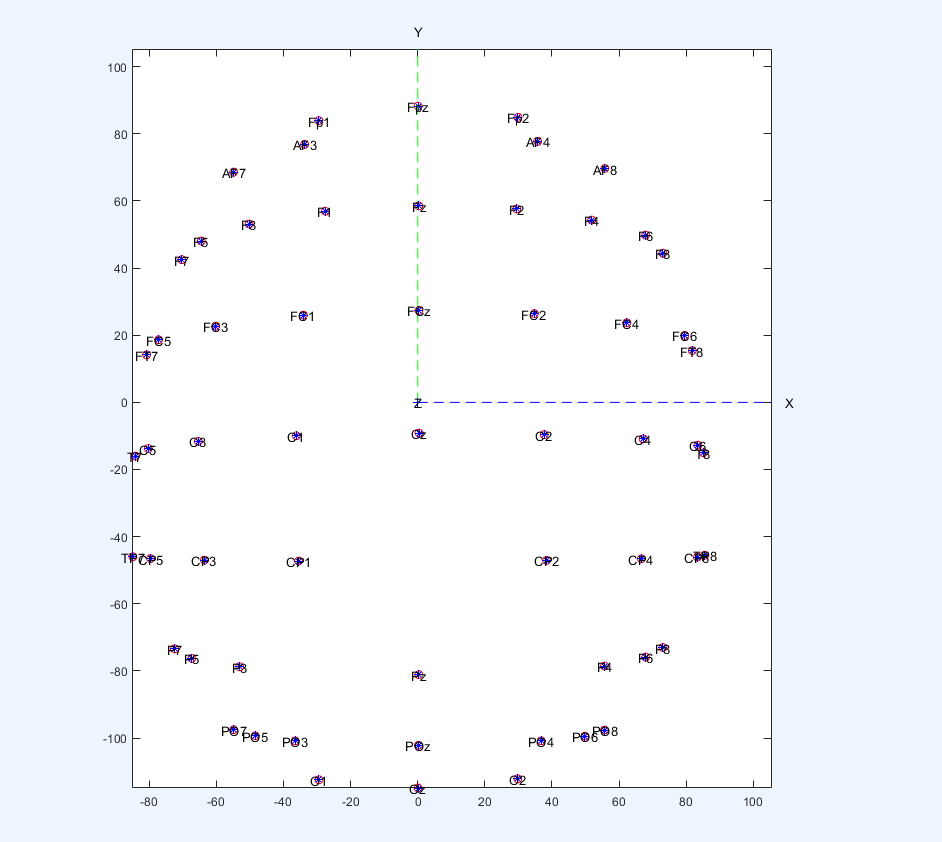
可以看到二维的并不是三维坐标二维的直接投影。
使用的布局文件是这个。
而是比较类似于透视投影的方式。

E:\tool\matlab\R2022a\toolbox\eeglab\plugins\dipfit\standard_BEM\elec\standard_1005.elc

EEGLAB 的标准电极文件
.elp 文件：EEGLAB 的电极位置文件，格式为 电极名称 X Y Z。
.set 文件：BESA 等软件的电极格式，包含坐标和蒙太奇信息

一个在脑图上的功能连接绘制

皮尔逊系数的功能连接绘制

import numpy as np
import matplotlib.pyplot as plt
import os
import numpy as np
import mne
from glob import glob
import matplotlib.pyplot as plt
from tqdm import tqdm  # for progress bars
import scipy.signal as signal
from scipy.stats import skew, kurtosis
import pickle
from mne import make_fixed_length_epochs

#此处使用了一个格式如下的epochs（150个批次，59通道，2s,128HZ采样率）
#(150, 59, 256)
# 可以从静息态数据直接获取，此处raw_data的通道信息也有用
pathdir=r"E:\data\301数据汇总\EEG\jxt_analysis\dataset\health\1"
file=r"processed_data.set"
path=os.path.join(pathdir, file)
raw_data = mne.io.read_raw_eeglab(path, preload=True)
epochs = make_fixed_length_epochs(raw_data, duration=1, overlap=0.5,preload=True)

#此处直接读取
def process_all_subjects(base_dir, save_path=None):
    health_dir = os.path.join(base_dir, "health")
    patient_dir = os.path.join(base_dir, "术前停药")
    
    # Find all subject folders
    health_subjects = [f.path for f in os.scandir(health_dir) if f.is_dir()]
    patient_subjects = [f.path for f in os.scandir(patient_dir) if f.is_dir()]
    return health_subjects, patient_subjects
Base_dir =  r"E:\data\301数据汇总\EEG\jxt_analysis\dataset"
h_data,p_data = process_all_subjects(Base_dir)
for i in h_data:
    epochfilepath = os.path.join(i,"epochs_data_59.npy")
    epochs_h = np.load(epochfilepath,allow_pickle=True)
def compute_adjacency_matrix(epoch_data, method='pearson'):
    """
    输入：一个 epoch 的 shape = (n_channels, n_times)
    输出：adjacency matrix, shape = (n_channels, n_channels)
    """
    if method == 'pearson':
        # shape: (n_channels, n_times)
        corr = np.corrcoef(epoch_data)
        # 对角线设为0，避免自连接
        np.fill_diagonal(corr, 0)
        return corr
    else:
        raise NotImplementedError(f"暂时只支持 pearson 方法")
def build_graph_from_adjacency(adj_matrix, threshold=None, top_k=None):
    """
    根据邻接矩阵构建图，可以选择设置阈值或保留top-k
    返回一个 NetworkX 的无向图
    """
    n_channels = adj_matrix.shape[0]
    G = nx.Graph()
    G.add_nodes_from(range(n_channels))
    
    if top_k is not None:
        # 保留每行的 top_k 连接
        for i in range(n_channels):
            top_indices = np.argsort(adj_matrix[i])[-top_k:]
            for j in top_indices:
                if adj_matrix[i, j] > 0.5:
                    G.add_edge(i, j, weight=adj_matrix[i, j])
    else:
        # 使用阈值
        for i in range(n_channels):
            for j in range(i+1, n_channels):
                if threshold is None or adj_matrix[i, j] >= threshold:
                    G.add_edge(i, j, weight=adj_matrix[i, j])
    return G

因为直接绘制连接，这些通道看起来会很乱，所以，限制布局为标准布局，再绘制功能网络。

#获取通道布局
def get_eeg_cap_positions(channel_names, montage_name='standard_1020'):
    montage = mne.channels.make_standard_montage(montage_name)
    pos_dict = montage.get_positions()['ch_pos']

    positions = {}
    for ch in channel_names:
        if ch in pos_dict:
            xyz = pos_dict[ch]
            positions[channel_names.index(ch)] = xyz[:2]  # 取前两个维度（x, y）
        else:
            print(f"⚠️ 通道 {ch} 不在 {montage_name} 中，跳过")
    return positions
 
#使用之前得到的raw_data获取的通道信息

此处给出和绘图相关的代码

import numpy as np
import matplotlib.pyplot as plt
import mne
import networkx as nx

def get_eeg_cap_positions(channel_names, montage):
    pos_3d = montage.get_positions()['ch_pos']
    pos = {}
    for idx, name in enumerate(channel_names):
        if name in pos_3d:
            xyz = pos_3d[name]
            # 透视投影
            x_proj = xyz[0] / (xyz[2] + 0.1)
            y_proj = xyz[1] / (xyz[2] + 0.1)
            pos[idx] = np.array([x_proj, y_proj])
        else:
            print(f"⚠️ {name} 不在 montage 中")
    return pos


def plot_graph_on_head(G, raw_or_epochs, title="EEG Connectivity Graph with Head Layout"):
    info = raw_or_epochs.info
    montage = info.get_montage()
    channel_names = info['ch_names']

    # 获取头图轮廓
    pos_3d = montage.get_positions()['ch_pos']
    pos_array = np.array([pos_3d[ch] for ch in channel_names])
    pos_2d = np.column_stack((pos_array[:, 0] / (pos_array[:, 2] + 0.1),
                              pos_array[:, 1] / (pos_array[:, 2] + 0.1)))

    sphere = np.array([0.0, 0.0, 0.04, 0.1108])
    outlines = mne.viz.topomap._make_head_outlines(sphere, pos_2d, outlines="head", clip_origin=(0.0, 0.0))

    # EEG通道位置，用于 networkx 画图
    node_pos = get_eeg_cap_positions(channel_names, montage)

    # 获取边权和节点度
    edge_weights = np.array([G[u][v]['weight'] for u, v in G.edges()])
    degrees = np.array([val for (_, val) in G.degree()])

    # Normalize 映射
    edge_widths = 1 + 4 * (edge_weights - edge_weights.min()) / (edge_weights.ptp() + 1e-6)
    edge_colors = edge_weights
    node_sizes = 100 + 300 * (degrees - degrees.min()) / (degrees.ptp() + 1e-6)
    node_colors = degrees

    # 创建图像 + layout 调整
    
    fig, ax = plt.subplots(figsize=(9, 9))
    ax.set_aspect("equal")
    ax.set_xlim(-1.5, 1.5)
    ax.set_ylim(-1.5, 1.5)
    ax.axis("off")  # 隐藏坐标轴

    # 绘制头部轮廓
    for key, val in outlines.items():
        if isinstance(val, (np.ndarray, list, tuple)):
            val = np.array(val)
            if val.shape[0] == 2:
                ax.plot(val[0]*10, val[1]*10, color="black", lw=2)

    # EEG 电极点 & 标签
    for i, (x, y) in enumerate(pos_2d):
        ax.scatter(x, y, color="gray", s=30, alpha=0.3)
        ax.annotate(text=channel_names[i],
                    xy=(x, y),
                    xytext=(2, 2),
                    textcoords="offset points",
                    fontsize=8,
                    color="black")

    # 🎯 绘制 Graph
    nodes = nx.draw_networkx_nodes(G, pos=node_pos, ax=ax,
                                   node_color=node_colors,
                                   node_size=node_sizes,
                                   cmap=plt.cm.plasma)

    edges = nx.draw_networkx_edges(G, pos=node_pos, ax=ax,
                                   edge_color=edge_colors,
                                   width=edge_widths,
                                   edge_cmap=plt.cm.viridis,
                                   alpha=0.8,
                                   connectionstyle="arc3,rad=0.4")  # 🎈曲线边！

    # 添加 colorbar（节点）
    sm_nodes = plt.cm.ScalarMappable(cmap=plt.cm.plasma,
                                     norm=plt.Normalize(vmin=degrees.min(), vmax=degrees.max()))
    sm_nodes.set_array([])
    cbar_ax_nodes = fig.add_axes([0.80, 0.15, 0.02, 0.35])
    cbar_nodes = fig.colorbar(sm_nodes, cax=cbar_ax_nodes)
    cbar_nodes.set_label("Node Degree", fontsize=10)
    cbar_nodes.ax.tick_params(labelsize=8)
    # 添加 colorbar（边）
    sm_edges = plt.cm.ScalarMappable(cmap=plt.cm.viridis,
                                     norm=plt.Normalize(vmin=edge_weights.min(), vmax=edge_weights.max()))
    sm_edges.set_array([])
    cbar_ax_edges = fig.add_axes([0.88, 0.15, 0.02, 0.35])
    cbar_edges = fig.colorbar(sm_edges, cax=cbar_ax_edges)
    cbar_edges.set_label("Edge Weight", fontsize=9)
    cbar_edges.ax.tick_params(labelsize=8)

    fig.suptitle(title, fontsize=14, y=0.95)
    # plt.title(title, fontsize=14)
    fig.subplots_adjust(left=0.1, right=0.5, top=0.88, bottom=0.1)

    plt.tight_layout()
    plt.show()

epoch = epochs_h[1]
adj = compute_adjacency_matrix(epoch)
G = build_graph_from_adjacency(adj, top_k=5)
#此处使用了raw_data提供了信息
plot_graph_on_head(G, raw_data, title=" Epoch 1 EEG Graph")

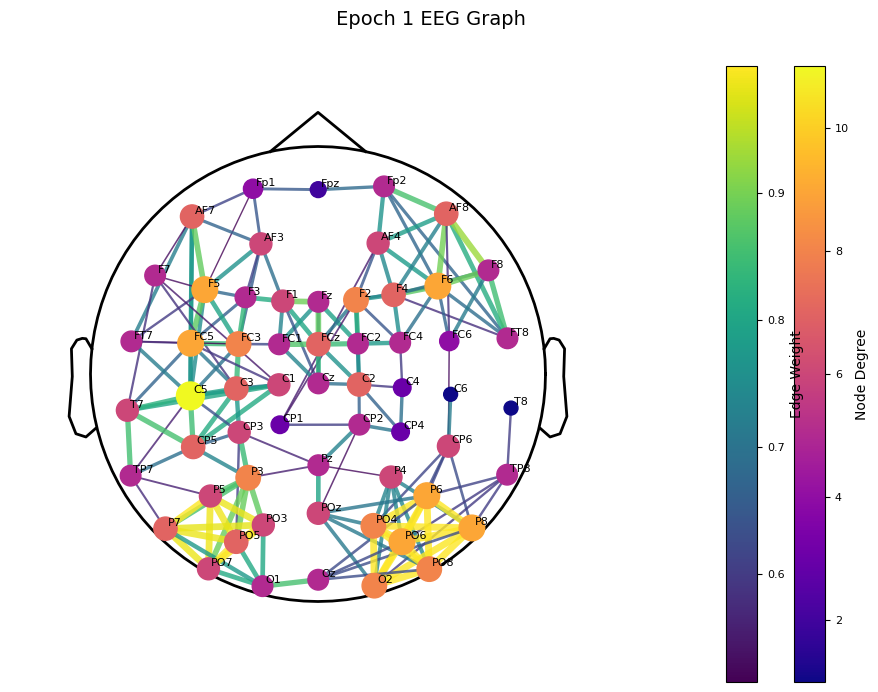
该图显示了脑电图的功能连接的图论指标，显示了边的权重和节点度。这个colorbar有些label重叠了。
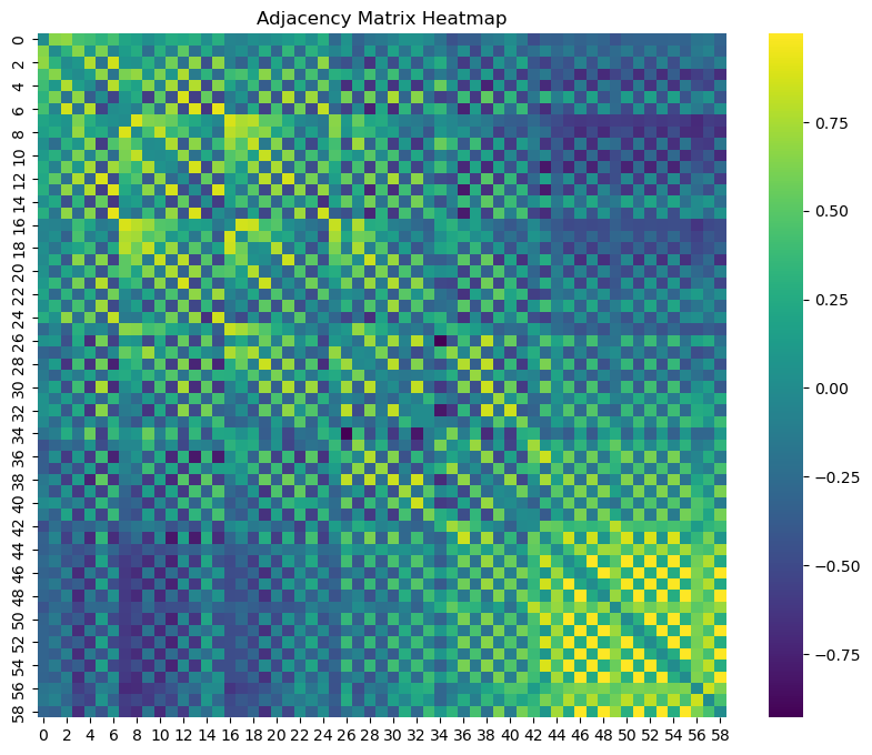
这个邻接矩阵的热图的绘制

import matplotlib.pyplot as plt
import seaborn as sns
epoch = epochs_h[1]
adj = compute_adjacency_matrix(epoch)
plt.figure(figsize=(10, 8))
sns.heatmap(adj, cmap='viridis', annot=False, fmt='.2f')
plt.title('Adjacency Matrix Heatmap')
plt.show()

总结

本文讨论了一些方法是如何实现这个电极图的绘制，如果想在这个图上使用更多自定义的代码绘制，可以基于此进行扩展。

后续再探讨一些可能的可视化方案：
比如可以把点的绘制部分，替换为其他的指标，同时，把一些网络指标或者功能连接指标，通过这个脑的图来绘制。

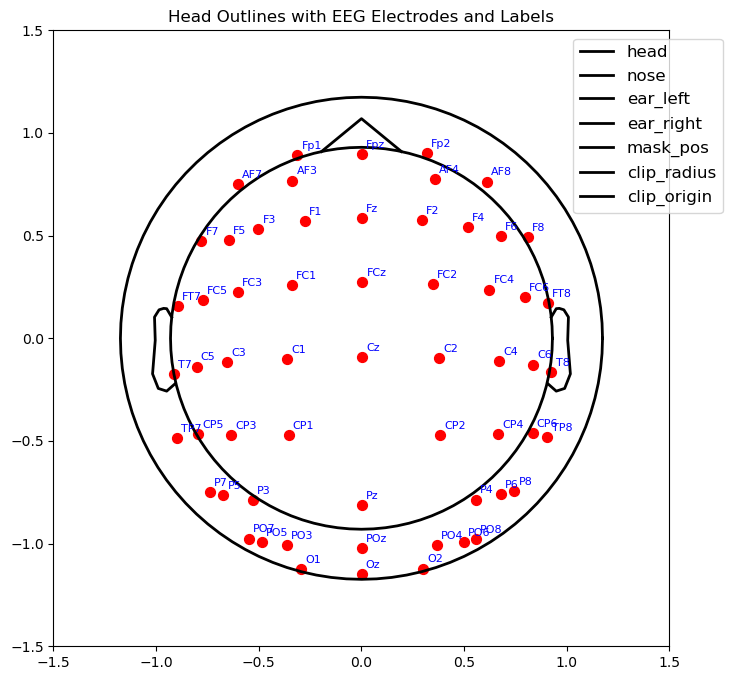
  ax.plot(val[0]*10, val[1]*10, color="black", lw=2, label=key)

import matplotlib.pyplot as plt
import numpy as np
import mne

# 生成头部轮廓
sphere = np.array([0.0, 0.0, 0.04, 0.1108])  # 适当增大半径
def perspective_projection(pos_3d, epsilon=0.1):
    positions = np.array(list(pos_3d.values()))
    x, y, z = positions[:,0], positions[:,1], positions[:,2]
    x_proj = x / (z + epsilon)
    y_proj = y / (z + epsilon)
    return np.column_stack((x_proj, y_proj))
info = raw_data.info  # 或 epochs.info
pos_3d = montage.get_positions()['ch_pos']
montage = info.get_montage()

pos = perspective_projection(pos_3d, epsilon=0.1)
head_outlines = mne.viz.topomap._make_head_outlines(sphere, pos, outlines="head", clip_origin=(0.0, 0.0))

# 创建绘图
fig, ax = plt.subplots(figsize=(8, 8))  # 让图像更清晰
ax.set_aspect("equal")
ax.set_xlim(-1.5, 1.5)
ax.set_ylim(-1.5, 1.5)

# 绘制头部轮廓
for key, val in head_outlines.items():
    if isinstance(val, (np.ndarray, list, tuple)):
        if isinstance(val, (list, tuple)):
            val = np.array(val) 
        if val.shape[0] == 2:
            print(f"绘制 {key}:")
            print(val[0], val[1])
            ax.plot(val[0]*10, val[1]*10, color="black", lw=2, label=key)
    else:
        print(f"Unexpected type for {key}: {type(val)}")

# # 绘制 EEG 通道
# ax.scatter(pos[:, 0], pos[:, 1], color="red", s=50, label="EEG Electrodes")
# 绘制 EEG 通道并添加名称
# 假设 pos 是二维数组（shape: (n_channels, 2)）
# 并且 info.ch_names 是通道名称列表
for i, (x, y) in enumerate(pos):
    # 绘制电极点
    ax.scatter(x , y , color="red", s=50)
    
    # 添加通道名称（注意坐标缩放）
    # 调整偏移量（dx, dy）以避免标签重叠
    ax.annotate(
        text=info.ch_names[i],  # 通道名称
        xy=(x , y ),   # 电极坐标（与 scatter 的坐标一致）
        xytext=(3, 3),         # 标签相对于电极点的偏移量（可调整）
        textcoords="offset points",  # 偏移量单位
        fontsize=8,            # 字体大小
        color="blue",          # 标签颜色
        ha="left",             # 水平对齐方式
        va="bottom"            # 垂直对齐方式
    )

ax.legend(loc='upper right', bbox_to_anchor=(1.1, 1), fontsize=12)

plt.title("Head Outlines with EEG Electrodes and Labels")
plt.show()