
Spatial Data Analysis(五):使用 `census` 包获取人口普查数据
本教程将帮助您学习如何使用 python 直接获取人口普查数据,以避免从人口普查网站下载的麻烦。安装“census”和“us”包。 “us”包提供了一些对 FIPS 代码的便捷查找。Import the packages首先,从此处获取人口普查 API 密钥。 这将要求您输入您的隶属关系和电子邮件。 然后您需要通过电子邮件激活您的 API 密钥。 然后您将得到一个长密钥字符串来替换我这里的字符串:
Spatial Data Analysis(五):使用 census 包获取人口普查数据
本教程将帮助您学习如何使用 python 直接获取人口普查数据,以避免从人口普查网站下载的麻烦。
安装“census”和“us”包。 “us”包提供了一些对 FIPS 代码的便捷查找。
pip install -q census
pip install -q us
Import the packages
import matplotlib.pyplot as plt
import pandas as pd
import geopandas as gpd
from census import Census
import us
首先,从此处获取人口普查 API 密钥。 这将要求您输入您的隶属关系和电子邮件。 然后您需要通过电子邮件激活您的 API 密钥。 然后您将得到一个长密钥字符串来替换我这里的字符串:
census_api_key = "0ed8bfc03db7e7bf1b990114c59b0840650c4fc7"

c = Census(census_api_key)
然后我们可以使用一个函数来自动下载人口普查数据并将其制作成格式良好的 Dataframe。
以下是获取变量的人口普查区级别数据的示例:
- 总人口 (B01003_001E)
- 每月住房费用中位数 (B25105_001E)
- 上班的交通工具(汽车、卡车、货车)(B08134_011E)
Lookup table for variables: https://api.census.gov/data/2019/acs/acs5/variables.html
# Sources: https://api.census.gov/data/2019/acs/acs5/variables.html

fl_census = c.acs5.state_county_tract(fields = ('NAME', 'B01003_001E', 'B25105_001E', 'B08134_001E'),
                                      state_fips = us.states.FL.fips,
                                      county_fips = "*",
                                      tract = "*",
                                      year = 2019)
Make the results a data frame.
fl_df = pd.DataFrame(fl_census)
fl_df.head()
| NAME | B01003_001E | B25105_001E | B08134_001E | state | county | tract | |
|---|---|---|---|---|---|---|---|
| 0 | Census Tract 2.11, Miami-Dade County, Florida | 2812.0 | 1456.0 | 1449.0 | 12 | 086 | 000211 |
| 1 | Census Tract 2.12, Miami-Dade County, Florida | 4709.0 | 1111.0 | 2157.0 | 12 | 086 | 000212 |
| 2 | Census Tract 2.13, Miami-Dade County, Florida | 5005.0 | 1260.0 | 2194.0 | 12 | 086 | 000213 |
| 3 | Census Tract 2.14, Miami-Dade County, Florida | 6754.0 | 1070.0 | 3194.0 | 12 | 086 | 000214 |
| 4 | Census Tract 1.28, Miami-Dade County, Florida | 3021.0 | 1322.0 | 1965.0 | 12 | 086 | 000128 |
让列名更直观。
fl_df = fl_df.rename(columns={
    "B01003_001E": "total_population",
    "B25105_001E": "monthly_housing_costs",
    "B08134_001E": "population_drive_to_work"
    })
fl_df.head()
| NAME | total_population | monthly_housing_costs | population_drive_to_work | state | county | tract | |
|---|---|---|---|---|---|---|---|
| 0 | Census Tract 2.11, Miami-Dade County, Florida | 2812.0 | 1456.0 | 1449.0 | 12 | 086 | 000211 |
| 1 | Census Tract 2.12, Miami-Dade County, Florida | 4709.0 | 1111.0 | 2157.0 | 12 | 086 | 000212 |
| 2 | Census Tract 2.13, Miami-Dade County, Florida | 5005.0 | 1260.0 | 2194.0 | 12 | 086 | 000213 |
| 3 | Census Tract 2.14, Miami-Dade County, Florida | 6754.0 | 1070.0 | 3194.0 | 12 | 086 | 000214 |
| 4 | Census Tract 1.28, Miami-Dade County, Florida | 3021.0 | 1322.0 | 1965.0 | 12 | 086 | 000128 |
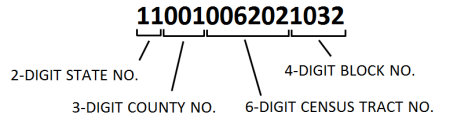
FIPS 代码
每个人口普查单位均由 FIPS(联邦信息处理标准)代码标识
从TIGER获取边界文件
一种直接从 TIGER 获取边界的快速且简单的方法。
首先我们需要知道我们想要的单位的 URL。
urls = us.states.FL.shapefile_urls()
urls.keys()
dict_keys(['tract', 'cd', 'county', 'state', 'zcta', 'block', 'blockgroup'])
urls['tract']
'https://www2.census.gov/geo/tiger/TIGER2010/TRACT/2010/tl_2010_12_tract10.zip'
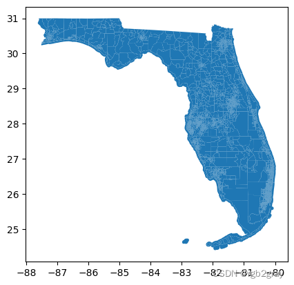
在这里,我们对佛罗里达州的人口普查区水平感兴趣。 *使用此方法您只能获得2010年TIGER方法。
fl_tract = gpd.read_file("https://www2.census.gov/geo/tiger/TIGER2010/TRACT/2010/tl_2010_12_tract10.zip")
fl_tract.plot()
<Axes: >
fl_tract.head()
| STATEFP10 | COUNTYFP10 | TRACTCE10 | GEOID10 | NAME10 | NAMELSAD10 | MTFCC10 | FUNCSTAT10 | ALAND10 | AWATER10 | INTPTLAT10 | INTPTLON10 | geometry | |
|---|---|---|---|---|---|---|---|---|---|---|---|---|---|
| 0 | 12 | 009 | 068300 | 12009068300 | 683 | Census Tract 683 | G5020 | S | 1886507 | 1893264 | +28.3410296 | -080.6080301 | POLYGON ((-80.60549 28.32007, -80.60687 28.320... |
| 1 | 12 | 009 | 068400 | 12009068400 | 684 | Census Tract 684 | G5020 | S | 1699567 | 6242872 | +28.3579064 | -080.6330330 | POLYGON ((-80.60214 28.35788, -80.60305 28.357... |
| 2 | 12 | 009 | 068601 | 12009068601 | 686.01 | Census Tract 686.01 | G5020 | S | 2981908 | 4187210 | +28.4044135 | -080.6306937 | POLYGON ((-80.64618 28.40506, -80.64619 28.405... |
| 3 | 12 | 009 | 068502 | 12009068502 | 685.02 | Census Tract 685.02 | G5020 | S | 1021413 | 549457 | +28.3860845 | -080.5984860 | POLYGON ((-80.59516 28.37972, -80.59896 28.379... |
| 4 | 12 | 009 | 068602 | 12009068602 | 686.02 | Census Tract 686.02 | G5020 | S | 3243209 | 1436745 | +28.4023088 | -080.6001604 | POLYGON ((-80.63220 28.40926, -80.62712 28.409... |
GeoDataFrame 具有 FIPS 代码,我们可以使用它来连接人口普查数据。 请注意,GEOID10 将州、县和地区代码连接在一起形成 11 位代码。
为了制作一致的键,我们需要在人口普查数据帧“fl_df”中创建一个新列,其结构与“fl_tract”中的“GEOID10”相同。
fl_df["GEOID10"] = fl_df["state"] + fl_df["county"] + fl_df["tract"]
fl_df["GEOID10"]
0       12086000211
1       12086000212
2       12086000213
3       12086000214
4       12086000128
           ...
4240    12019031200
4241    12019030801
4242    12019030902
4243    12019030301
4244    12019031400
Name: GEOID10, Length: 4245, dtype: object
基于相同的密钥“GEOID10”合并两个数据帧。
fl_tract_df = pd.merge(fl_tract, fl_df,on="GEOID10")
fl_tract_df.head()
| STATEFP10 | COUNTYFP10 | TRACTCE10 | GEOID10 | NAME10 | NAMELSAD10 | MTFCC10 | FUNCSTAT10 | ALAND10 | AWATER10 | INTPTLAT10 | INTPTLON10 | geometry | NAME | total_population | monthly_housing_costs | population_drive_to_work | state | county | tract | |
|---|---|---|---|---|---|---|---|---|---|---|---|---|---|---|---|---|---|---|---|---|
| 0 | 12 | 009 | 068300 | 12009068300 | 683 | Census Tract 683 | G5020 | S | 1886507 | 1893264 | +28.3410296 | -080.6080301 | POLYGON ((-80.60549 28.32007, -80.60687 28.320... | Census Tract 683, Brevard County, Florida | 2790.0 | 1068.0 | 675.0 | 12 | 009 | 068300 |
| 1 | 12 | 009 | 068400 | 12009068400 | 684 | Census Tract 684 | G5020 | S | 1699567 | 6242872 | +28.3579064 | -080.6330330 | POLYGON ((-80.60214 28.35788, -80.60305 28.357... | Census Tract 684, Brevard County, Florida | 2001.0 | 948.0 | 606.0 | 12 | 009 | 068400 |
| 2 | 12 | 009 | 068601 | 12009068601 | 686.01 | Census Tract 686.01 | G5020 | S | 2981908 | 4187210 | +28.4044135 | -080.6306937 | POLYGON ((-80.64618 28.40506, -80.64619 28.405... | Census Tract 686.01, Brevard County, Florida | 1978.0 | 898.0 | 771.0 | 12 | 009 | 068601 |
| 3 | 12 | 009 | 068502 | 12009068502 | 685.02 | Census Tract 685.02 | G5020 | S | 1021413 | 549457 | +28.3860845 | -080.5984860 | POLYGON ((-80.59516 28.37972, -80.59896 28.379... | Census Tract 685.02, Brevard County, Florida | 2492.0 | 848.0 | 1190.0 | 12 | 009 | 068502 |
| 4 | 12 | 009 | 068602 | 12009068602 | 686.02 | Census Tract 686.02 | G5020 | S | 3243209 | 1436745 | +28.4023088 | -080.6001604 | POLYGON ((-80.63220 28.40926, -80.62712 28.409... | Census Tract 686.02, Brevard County, Florida | 4272.0 | 957.0 | 1458.0 | 12 | 009 | 068602 |
fl_tract_df.plot(column="monthly_housing_costs",legend=True)
<Axes: >
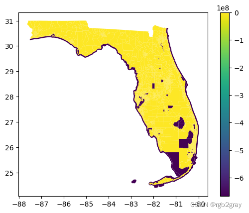
发生了什么? 为什么有些值真的很奇怪?
fl_tract_df.monthly_housing_costs.hist()
<Axes: >
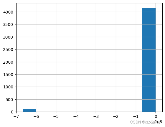
似乎有一些缺失值编码为-666666666.0,导致地图倾斜。
import numpy as np
fl_tract_df.monthly_housing_costs.to_string()
我们能做的就是将缺失值设为NA。
fl_tract_df = fl_tract_df.replace(-666666666.0, np.nan)
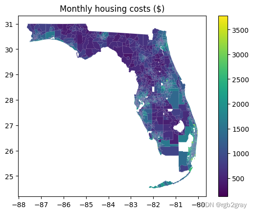
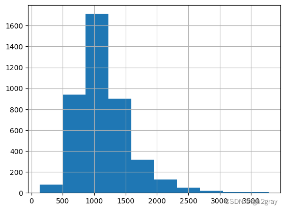
现在看起来很正常。 请注意,该值代表以美元计算的住房成本。
fl_tract_df.plot(column="monthly_housing_costs",legend=True)
plt.title("Monthly housing costs ($)")
Text(0.5, 1.0, 'Monthly housing costs ($)')
fl_tract_df["monthly_housing_costs"].hist()
<Axes: >
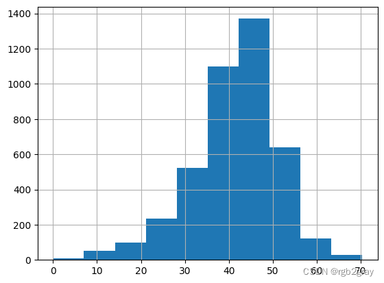
现在让我们看看另一个变量,人口的工作动力。 在这里,我们可以计算开车上班的人的百分比,并在数据框中创建一个新列。
fl_tract_df["pct_drive"] = fl_tract_df["population_drive_to_work"]/fl_tract_df["total_population"]*100
fl_tract_df["pct_drive"].hist()
<Axes: >
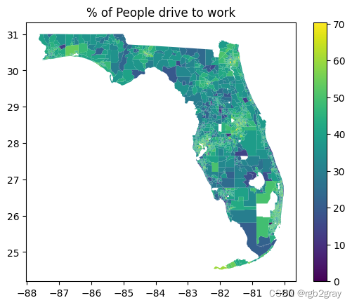
fl_tract_df.plot(column="pct_drive",legend=True)
plt.title("% of People drive to work")
Text(0.5, 1.0, '% of People drive to work')
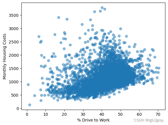
显示两个变量之间正相关的简单散点图。
plt.scatter(fl_tract_df["pct_drive"], fl_tract_df["monthly_housing_costs"],alpha=0.5)
plt.xlabel("% Drive to Work")
plt.ylabel("Monthly Housing Costs")
Text(0, 0.5, 'Monthly Housing Costs')

GitCode 天启AI是一款由 GitCode 团队打造的智能助手,基于先进的LLM(大语言模型)与多智能体 Agent 技术构建,致力于为用户提供高效、智能、多模态的创作与开发支持。它不仅支持自然语言对话,还具备处理文件、生成 PPT、撰写分析报告、开发 Web 应用等多项能力,真正做到“一句话,让 Al帮你完成复杂任务”。
更多推荐


 20
20 0
0- 0


 已为社区贡献5条内容

所有评论(0)