
Applied Spatial Statistics(八):GWR 和 MGWR 示例
我们经常会观察到 GWR 模型的残差具有较低的 Moran’s I 值,这表明已考虑了空间结构。局部截距是一种内在背景效应,例如,表明有多少影响可以归因于“位置”。在 GWR 或 MGWR 中,我们经常建议对独立变量和因变量进行标准化。中获得,它返回一个 n x p 数组,其中 p 是模型中的预测变量的数量(包括截距)。这种方法的好处是,获得的系数变得“无单位”,允许跨变量和位置比较变量重要性。这
Applied Spatial Statistics(八):GWR 和 MGWR 示例
这是一个基本示例笔记本,演示了如何校准 GWR 或 MGWR 模型。
安装
pip install mgwr
#pip install mgwr
Load packages
import numpy as np
import matplotlib.pyplot as plt
import geopandas as gpd
import pandas as pd
import libpysal as ps
from libpysal.weights import Queen
from esda.moran import Moran

#MGWR functions
from mgwr.gwr import GWR,MGWR
from mgwr.sel_bw import Sel_BW
Load voting dataset
voting = pd.read_csv('https://raw.github.com/Ziqi-Li/gis5122/master/data/voting_2020.csv')

voting[['median_income']] = voting[['median_income']]/10000
shp = gpd.read_file("https://raw.github.com/Ziqi-Li/gis5122/master/data/us_counties.geojson")
#Merge the shapefile with the voting data by the common county_id
shp_voting = shp.merge(voting, on ="county_id")

#Dissolve the counties to obtain boundary of states, used for mapping
state = shp_voting.dissolve(by='STATEFP').geometry.boundary
variable_names = ['sex_ratio', 'pct_black', 'pct_hisp',
                  'pct_bach', 'median_income','ln_pop_den']


y = shp_voting[['new_pct_dem']].values

X = shp_voting[variable_names].values
在 GWR 或 MGWR 中,我们经常建议对独立变量和因变量进行标准化。这里的标准化意味着我们减去平均值并除以标准化值。
这种方法的好处是,获得的系数变得“无单位”,允许跨变量和位置比较变量重要性。
X = (X - X.mean(axis=0))/X.std(axis=0)
y = (y - y.mean(axis=0))/y.std(axis=0)
我们需要将坐标输入到 GWR。
coords = shp_voting[['proj_X', 'proj_Y']].values
两步拟合 GWR 模型
- 选择最佳带宽
- 使用最佳带宽拟合 GWR 模型
默认内核是自适应(最近邻居数)双平方。
gwr_selector = Sel_BW(coords, y, X)

gwr_bw = gwr_selector.search(verbose=True)

print("Selected optimal bandwidth is:", gwr_bw)
Bandwidth:  1219.0 , score:  4058.94
Bandwidth:  1938.0 , score:  4614.76
Bandwidth:  774.0 , score:  3557.79
Bandwidth:  499.0 , score:  3140.51
Bandwidth:  329.0 , score:  2802.09
Bandwidth:  224.0 , score:  2530.12
Bandwidth:  159.0 , score:  2375.52
Bandwidth:  119.0 , score:  2310.56
Bandwidth:  94.0 , score:  2291.48
Bandwidth:  79.0 , score:  2297.64
Bandwidth:  104.0 , score:  2296.46
Bandwidth:  89.0 , score:  2289.15
Bandwidth:  85.0 , score:  2289.31
Bandwidth:  91.0 , score:  2289.59
Bandwidth:  87.0 , score:  2291.76
Selected optimal bandwidth is: 89.0
使用最佳 bw 拟合模型
gwr_results = GWR(coords, y, X, bw=gwr_bw,name_x=variable_names).fit()
GWR 输出摘要
gwr_results.summary()
===========================================================================
Model type                                                         Gaussian
Number of observations:                                                3103
Number of covariates:                                                     7

Global Regression Results
---------------------------------------------------------------------------
Residual sum of squares:                                           1213.006
Log-likelihood:                                                   -2945.693
AIC:                                                               5905.385
AICc:                                                              5907.432
BIC:                                                             -23679.220
R2:                                                                   0.609
Adj. R2:                                                              0.608

Variable                              Est.         SE  t(Est/SE)    p-value
------------------------------- ---------- ---------- ---------- ----------
Intercept                           -0.000      0.011     -0.000      1.000
sex_ratio                            0.004      0.012      0.350      0.727
pct_black                            0.434      0.013     34.477      0.000
pct_hisp                             0.206      0.011     18.026      0.000
pct_bach                             0.574      0.017     34.171      0.000
median_income                       -0.144      0.017     -8.403      0.000
ln_pop_den                           0.227      0.014     16.502      0.000

Geographically Weighted Regression (GWR) Results
---------------------------------------------------------------------------
Spatial kernel:                                           Adaptive bisquare
Bandwidth used:                                                      89.000

Diagnostic information
---------------------------------------------------------------------------
Residual sum of squares:                                            246.915
Effective number of parameters (trace(S)):                          548.884
Degree of freedom (n - trace(S)):                                  2554.116
Sigma estimate:                                                       0.311
Log-likelihood:                                                    -475.996
AIC:                                                               2051.760
AICc:                                                              2289.148
BIC:                                                               5373.125
R2:                                                                   0.920
Adjusted R2:                                                          0.903
Adj. alpha (95%):                                                     0.001
Adj. critical t value (95%):                                          3.419

Summary Statistics For GWR Parameter Estimates
---------------------------------------------------------------------------
Variable                   Mean        STD        Min     Median        Max
-------------------- ---------- ---------- ---------- ---------- ----------
Intercept                -0.036      0.760     -2.428     -0.038      5.779
sex_ratio                -0.016      0.098     -0.463     -0.023      0.449
pct_black                 0.534      0.867     -5.910      0.608      9.513
pct_hisp                  0.327      0.373     -1.335      0.304      3.561
pct_bach                  0.406      0.236     -0.507      0.404      1.249
median_income            -0.191      0.190     -0.885     -0.176      0.289
ln_pop_den                0.249      0.253     -0.562      0.219      1.416
===========================================================================
局部估计值可以从gwr_results.params中获得,它返回一个 n x p 数组,其中 p 是模型中的预测变量的数量(包括截距)。
variable_names
['sex_ratio',
 'pct_black',
 'pct_hisp',
 'pct_bach',
 'median_income',
 'ln_pop_den']
gwr_results.params[:,4]
array([ 0.56501565,  0.61552673,  0.42141522, ..., -0.09090834,
        0.75477483,  0.39401467])
from matplotlib import colors
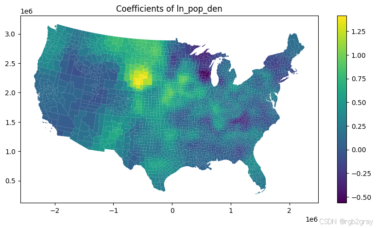
ax = shp_voting.plot(column=gwr_results.params[:,6],figsize=(10,5),legend=True,
linewidth=0.0,aspect=1)
plt.title("Coefficients of ln_pop_den",fontsize=12)
Text(0.5, 1.0, 'Coefficients of ln_pop_den')
编写一些绘图代码,将参数估计表面全部可视化。我们需要将 GWR 结果与县 GeoDataFrame 连接起来。
from mpl_toolkits.axes_grid1 import make_axes_locatable
from mgwr.utils import shift_colormap,truncate_colormap
from matplotlib import cm,colors

def param_plots(result, gdf, names=[], filter_t=False,figsize=(10, 10)):

    #Size of the plot. Here we have a 2 by 2 layout.
    k = gwr_results.k

    fig, axs = plt.subplots(int(k/2)+1, 2, figsize=figsize)
    axs = axs.ravel()

    #The max and min values of the color bar.
    vmin = -0.8
    vmax = 0.8

    cmap = cm.get_cmap("bwr_r")
    norm = colors.BoundaryNorm(np.arange(-0.8,0.9,0.1),ncolors=256)

    for j in range(k):

        pd.concat([gdf,pd.DataFrame(np.hstack([result.params,result.bse]))],axis=1).plot(ax=axs[j],column=j,vmin=vmin,vmax=vmax,
                                                                                         cmap=cmap,norm=norm,linewidth=0.1,edgecolor='white',aspect=1)
        axs[j].set_title("Parameter estimates of \n" + names[j],fontsize=10)

        if filter_t:
            rslt_filtered_t = result.filter_tvals()
            if (rslt_filtered_t[:,j] == 0).any():
                gdf[rslt_filtered_t[:,j] == 0].plot(color='lightgrey', ax=axs[j],linewidth=0.1,edgecolor='white',aspect=1)

        plt.axis('off')

    fig = axs[j].get_figure()
    cax = fig.add_axes([0.99, 0.2, 0.025, 0.6])
    sm = plt.cm.ScalarMappable(cmap=cmap,norm=norm)
    # fake up the array of the scalar mappable. Urgh...
    sm._A = []
    fig.colorbar(sm, cax=cax)
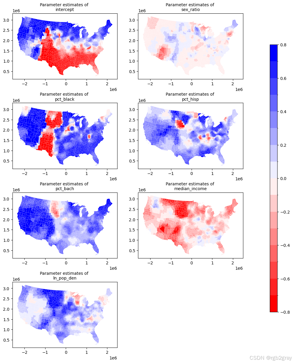
以下是从 GWR 获得的参数估计图。每个图代表每个预测因子与 PctBach 之间的空间关系。
- 正(负)关系以红色(蓝色)显示。
- 较强(较弱)的关系颜色较深(较浅)。
param_plots(gwr_results, shp_voting, names=['intercept'] + variable_names,figsize = (10,15))
/var/folders/mp/9px298sd6vs8xccb_3sql0dr0000gp/T/ipykernel_19922/1374554983.py:17: MatplotlibDeprecationWarning: The get_cmap function was deprecated in Matplotlib 3.7 and will be removed two minor releases later. Use ``matplotlib.colormaps[name]`` or ``matplotlib.colormaps.get_cmap(obj)`` instead.
  cmap = cm.get_cmap("bwr_r")
现在让我们检查一下 GWR 模型的残差。
#Here we use the Queen contiguity
w = Queen.from_dataframe(shp_voting)

#row standardization
w.transform = 'R'

residual_moran = Moran(gwr_results.resid_response.reshape(-1), w)
residual_moran.I
/var/folders/mp/9px298sd6vs8xccb_3sql0dr0000gp/T/ipykernel_14666/2963299590.py:2: FutureWarning: `use_index` defaults to False but will default to True in future. Set True/False directly to control this behavior and silence this warning
  w = Queen.from_dataframe(shp_voting)
/Users/ziqili/anaconda3/lib/python3.11/site-packages/libpysal/weights/weights.py:224: UserWarning: The weights matrix is not fully connected:
 There are 3 disconnected components.
 There are 2 islands with ids: 2441, 2701.
  warnings.warn(message)


('WARNING: ', 2441, ' is an island (no neighbors)')
('WARNING: ', 2701, ' is an island (no neighbors)')


0.1142496644549166
我们经常会观察到 GWR 模型的残差具有较低的 Moran’s I 值,这表明已考虑了空间结构。局部截距是一种内在背景效应,例如,表明有多少影响可以归因于“位置”。
GWR 推断
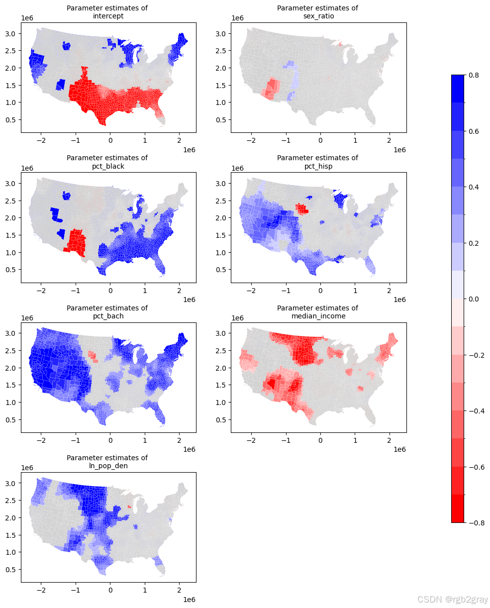
局部系数显著性
以下是**显著性(p<0.05)**参数估计值的图。显著性检验已调整以解决多重检验问题(Bonferroni)。
不显著的参数用灰色遮盖。
这是通过 param_plots() 函数中的 result.filter_tvals() 完成的。
param_plots(gwr_results, shp_voting, names=['intercept'] + variable_names,figsize = (10,15), filter_t=True)
/var/folders/mp/9px298sd6vs8xccb_3sql0dr0000gp/T/ipykernel_14666/3391375418.py:17: MatplotlibDeprecationWarning: The get_cmap function was deprecated in Matplotlib 3.7 and will be removed two minor releases later. Use ``matplotlib.colormaps[name]`` or ``matplotlib.colormaps.get_cmap(obj)`` instead.
  cmap = cm.get_cmap("bwr_r")
两步拟合 MGWR 模型
- 寻找最佳带宽
- 使用最佳带宽拟合 MGWR 模型
注意:当数据超过 5,000 条记录时,MGWR 会变慢。
%%time
mgwr_selector = Sel_BW(coords, y, X,multi=True)
mgwr_bw = mgwr_selector.search(verbose=True)

print("Selected optimal bandwidth is:", gwr_bw)
mgwr_results = MGWR(coords, y, X, selector=mgwr_selector,name_x=variable_names).fit()
mgwr_results.summary()
===========================================================================
Model type                                                         Gaussian
Number of observations:                                                3103
Number of covariates:                                                     7

Global Regression Results
---------------------------------------------------------------------------
Residual sum of squares:                                           1213.006
Log-likelihood:                                                   -2945.693
AIC:                                                               5905.385
AICc:                                                              5907.432
BIC:                                                             -23679.220
R2:                                                                   0.609
Adj. R2:                                                              0.608

Variable                              Est.         SE  t(Est/SE)    p-value
------------------------------- ---------- ---------- ---------- ----------
Intercept                           -0.000      0.011     -0.000      1.000
sex_ratio                            0.004      0.012      0.350      0.727
pct_black                            0.434      0.013     34.477      0.000
pct_hisp                             0.206      0.011     18.026      0.000
pct_bach                             0.574      0.017     34.171      0.000
median_income                       -0.144      0.017     -8.403      0.000
ln_pop_den                           0.227      0.014     16.502      0.000

Multi-Scale Geographically Weighted Regression (MGWR) Results
---------------------------------------------------------------------------
Spatial kernel:                                           Adaptive bisquare
Criterion for optimal bandwidth:                                       AICc
Score of Change (SOC) type:                                     Smoothing f
Termination criterion for MGWR:                                       1e-05

MGWR bandwidths
---------------------------------------------------------------------------
Variable             Bandwidth      ENP_j   Adj t-val(95%)   Adj alpha(95%)
Intercept               44.000    140.857            3.575            0.000
sex_ratio             1934.000      3.412            2.442            0.015
pct_black               44.000    136.138            3.566            0.000
pct_hisp              1275.000      3.610            2.463            0.014
pct_bach               180.000     31.072            3.157            0.002
median_income           44.000    146.952            3.587            0.000
ln_pop_den             228.000     21.568            3.049            0.002

Diagnostic information
---------------------------------------------------------------------------
Residual sum of squares:                                            224.288
Effective number of parameters (trace(S)):                          483.608
Degree of freedom (n - trace(S)):                                  2619.392
Sigma estimate:                                                       0.293
Log-likelihood:                                                    -326.874
AIC:                                                               1622.964
AICc:                                                              1802.784
BIC:                                                               4550.059
R2                                                                    0.928
Adjusted R2                                                           0.914

Summary Statistics For MGWR Parameter Estimates
---------------------------------------------------------------------------
Variable                   Mean        STD        Min     Median        Max
-------------------- ---------- ---------- ---------- ---------- ----------
Intercept                -0.111      0.542     -1.276     -0.055      0.955
sex_ratio                -0.022      0.007     -0.038     -0.021     -0.010
pct_black                 0.497      0.322     -0.979      0.580      1.109
pct_hisp                  0.285      0.027      0.227      0.290      0.329
pct_bach                  0.401      0.143     -0.098      0.397      0.744
median_income            -0.197      0.168     -1.069     -0.170      0.342
ln_pop_den                0.243      0.120      0.040      0.244      0.505
===========================================================================
#Here we use the Queen contiguity
w = Queen.from_dataframe(shp_voting)

#row standardization
w.transform = 'R'

residual_moran = Moran(mgwr_results.resid_response.reshape(-1), w)
residual_moran.I
('WARNING: ', 2441, ' is an island (no neighbors)')
('WARNING: ', 2701, ' is an island (no neighbors)')


/var/folders/mp/9px298sd6vs8xccb_3sql0dr0000gp/T/ipykernel_14666/3541487640.py:2: FutureWarning: `use_index` defaults to False but will default to True in future. Set True/False directly to control this behavior and silence this warning
  w = Queen.from_dataframe(shp_voting)
/Users/ziqili/anaconda3/lib/python3.11/site-packages/libpysal/weights/weights.py:224: UserWarning: The weights matrix is not fully connected:
 There are 3 disconnected components.
 There are 2 islands with ids: 2441, 2701.
  warnings.warn(message)


0.01835193713566798
param_plots(mgwr_results, shp_voting, names=['intercept'] + variable_names,figsize = (10,15), filter_t=True)
/var/folders/mp/9px298sd6vs8xccb_3sql0dr0000gp/T/ipykernel_14666/3391375418.py:17: MatplotlibDeprecationWarning: The get_cmap function was deprecated in Matplotlib 3.7 and will be removed two minor releases later. Use ``matplotlib.colormaps[name]`` or ``matplotlib.colormaps.get_cmap(obj)`` instead.
  cmap = cm.get_cmap("bwr_r")
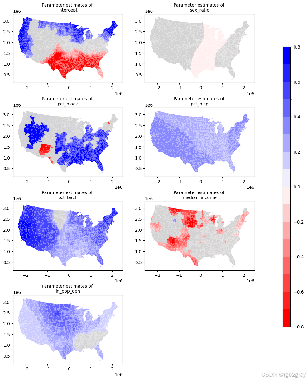
We can see that the relationships will vary at different spatial scales.
OLS vs. GWR vs. MGWR
From the comparison, we can clearly see an advantage of MGWR over GWR by allowing the bandwidth to vary across covariates.
| Metric | OLS | GWR | MGWR |
|---|---|---|---|
| R2 | 0.609 | 0.920 | 0.928 |
| AICc | 5907.4 | 2289.1 | 1802.7 |
| Moran’s I of residuals | 0.60 | 0.11 | 0.018 |
relationships will vary at different spatial scales.
OLS vs. GWR vs. MGWR
From the comparison, we can clearly see an advantage of MGWR over GWR by allowing the bandwidth to vary across covariates.
| Metric | OLS | GWR | MGWR |
|---|---|---|---|
| R2 | 0.609 | 0.920 | 0.928 |
| AICc | 5907.4 | 2289.1 | 1802.7 |
| Moran’s I of residuals | 0.60 | 0.11 | 0.018 |

GitCode 天启AI是一款由 GitCode 团队打造的智能助手,基于先进的LLM(大语言模型)与多智能体 Agent 技术构建,致力于为用户提供高效、智能、多模态的创作与开发支持。它不仅支持自然语言对话,还具备处理文件、生成 PPT、撰写分析报告、开发 Web 应用等多项能力,真正做到“一句话,让 Al帮你完成复杂任务”。
更多推荐


 10
10 0
0- 0


 已为社区贡献5条内容

所有评论(0)