
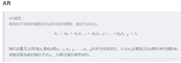
随机序列模型
文章目录一、随机序列1、平稳序列2、非平稳随机序列二、ARMA模型1、自回归模型2、滑动平均模型3、自回归滑动平均模型一、随机序列1、平稳序列2、非平稳随机序列二、ARMA模型1、自回归模型2、滑动平均模型3、自回归滑动平均模型时间序列平稳性_ADF检验...
·
文章目录
时间序列
- 白噪声
- 平稳的非白噪声序列(AR\MA\ARMA)
- 非平稳序列(差分——>ARIMA)
- 单变量ts(ARMA——>GARCH)
- 多变量(VAR——>MGARCH)
平稳性检验 - 单位根检验
- ACF和PACF(截尾0、拖尾-衰减但没到0)
一、随机序列
1、平稳序列

2、非平稳随机序列

二、ARMA模型
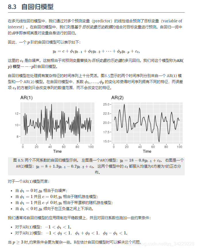
1、自回归模型


import numpy as np
import matplotlib.pyplot as plt
import pandas as pd
from statsmodels.graphics.tsaplots import plot_acf
from statsmodels.graphics.tsaplots import plot_pacf
ARMA模型预测时间序列
创建AR(2)模型
# 创建一个2阶的AR模型
def creat_ar(ar, length):
    for i in range(length):
        w = np.random.normal(loc=0.0, scale=1.0,size = length)
        y_0, y_1 = ar[i], ar[i + 1]
        y_2 =  0.8 * y_1 - 0.7 * y_0 + w[i]
        ar.append(y_2)
    return ar
ar = [0.1, 0.7]
creat_ar(ar, 1000)
[0.1,
 0.7,
 0.12840854214460806,
 ...]
创建一个MA(2)模型
def creat_ma(ma, length):
    delta_t = np.random.normal(loc=0.0, scale=1.0, size=length + 2)
    for i in range(length):
        y_1 = delta_t[i + 2] - delta_t[i + 1] + 0.8 * delta_t[i]
        ma.append(y_1)
    return ma

ma = []
creat_ma(ma, 1000)
[-1.3984698355642537,
 1.4199886006926872,
...
 -0.5279371496558356]
# 可视化
plt.figure()
plt.title("AR(2)")
plt.plot(ar)
plt.show()
plt.figure()
plt.title("MA(2)")
plt.plot(ma)
plt.show()


ADF检验
# adf 稳定性检验
def stationarity_test(dataset, number):
    data = dataset.copy()
    data = data[: len(data) - number]  # 不检测最后number个数据
    # 平稳性检测
    from statsmodels.tsa.stattools import adfuller as ADF
    diff = 0
    adf = ADF(data)
    while adf[1] > 0.05:
        diff = diff + 1
        adf = ADF(data.diff(diff).dropna())  # 对序列求1阶差分后,判断其是否平稳
    print(u'原始序列经过%s阶差分后归于平稳,p值为%s' % (diff, adf[1]))
    return adf


adf = stationarity_test(ar, 0)
print("adf:", adf)
原始序列经过0阶差分后归于平稳,p值为2.9074190502342907e-14
adf: (-8.746832168637235, 2.9074190502342907e-14, 13, 988, {'1%': -3.4369860032923145, '5%': -2.8644697838498376, '10%': -2.5683299626694422}, 2773.7293591490547)
白噪声检验
# 白噪声检验
def whitenoise_test(dataset, number):
    data = dataset.copy()
    data = data[: len(data) - number]  # 不使用最后number个数据
    # 白噪声检测
    from statsmodels.stats.diagnostic import acorr_ljungbox
    lb, p = acorr_ljungbox(data, lags=1)
    if p < 0.05:
        print(u'原始序列为非白噪声序列,对应的p值为:%s' % p)
    else:
        print(u'原始该序列为白噪声序列,对应的p值为:%s' % p)
    lb, p = acorr_ljungbox(data.diff().dropna(), lags=1)
    if p < 0.05:
        print(u'一阶差分序列为非白噪声序列,对应的p值为:%s' % p)
    else:
        print(u'一阶差分该序列为白噪声序列,对应的p值为:%s' % p)


whitenoise_test(pd.Series(ar), 0)
原始序列为非白噪声序列,对应的p值为:[7.40542966e-49]
一阶差分序列为非白噪声序列,对应的p值为:[4.24539224e-15]
ACF图和PACF图
# 第一步:先检查平稳序列的自相关图和偏自相关图
fig = plt.figure(figsize=(12, 8))
ax1 = fig.add_subplot(211)
fig = plot_acf(ar, lags=40, ax=ax1)
# lags 表示滞后的阶数
# 第二步:下面分别得到acf 图和pacf 图
ax2 = fig.add_subplot(212)
fig = plot_pacf(ar, lags=40, ax=ax2)

热力图定阶
热力图定阶结果为ARMA(2,10)
#     import seaborn as sns #热力图
#     import itertools
#     from statsmodels.tsa.arima_model import ARMA

#     #设置遍历循环的初始条件,以热力图的形式展示,跟AIC定阶作用一样
#     p_min = 0
#     q_min = 0
#     p_max = 5
#     q_max = 5
#     # 创建Dataframe,以BIC准则
#     results_aic = pd.DataFrame(index=['AR{}'.format(i) \
#                                for i in range(p_min,p_max+1)],\
#             columns=['MA{}'.format(i) for i in range(q_min,q_max+1)])
#     # itertools.product 返回p,q中的元素的笛卡尔积的元组
#     for p,q in itertools.product(range(p_min,p_max+1),\
#                                    range(q_min,q_max+1)):
# #         print(p,q)
#         if p==0 and q==0:
#             results_aic.loc['AR{}'.format(p), 'MA{}'.format(q)] = np.nan
#             continue
#         try:

#             model = ARMA(ar, order=(p,q))
# #             print("训练模型")
#             results = model.fit()
#             #返回不同pq下的model的BIC值
#             results_aic.loc['AR{}'.format(p), 'MA{}'.format(q)] = results.aic
#         except:
#             continue
#     results_aic = results_aic[results_aic.columns].astype(float)
#     #print(results_bic)

#     fig, ax = plt.subplots(figsize=(10, 8))
#     ax = sns.heatmap(results_aic,
#                  #mask=results_aic.isnull(),
#                  ax=ax,
#                  annot=True, #将数字显示在热力图上
#                  fmt='.2f',
#                  )
#     ax.set_title('AIC')
#     plt.show()
拟合ARMA(2,10)和预测
from statsmodels.tsa.arima_model import ARMA
from statsmodels.tsa.ar_model import AR
def plot_results(predicted_data, true_data):
  fig = plt.figure(facecolor='white',figsize=(10,5))
  plt.figure()
  plt.plot(np.arange(len(true_data)),true_data, label='True Data')
  plt.plot(np.arange(len(true_data)),predicted_data, label='Prediction')
  plt.legend()
  plt.show()


def arma_predict(data,number):
  train = data[:-72]
  test = data[-72:]

  model = ARMA(train,order=(2,10))
  result_arma = model.fit(maxlag=10, ic='aic', trend='nc') # disp=-1, method='css'
  predict = result_arma.predict(len(data)-72,len(data)-1)
  #RMSE = np.sqrt(((predict-data[len(data)-number-1:])**2).sum()/(number+1))
  plot_results(predict,test)
  return predict,test


p,t = arma_predict(ar,72)
print(p,t)

[ 4.93338218e-01  9.70453432e-01  5.21605850e-01 -2.52319478e-01
 -6.15976064e-01 -2.88352786e-01  1.09334879e-01  3.00866168e-01
  2.45437776e-01  2.62972589e-02 -1.61168837e-01 -1.94441833e-01
 -8.55881203e-02  5.77198278e-02  1.28471296e-01  9.42185033e-02
  2.56147065e-03 -7.00087112e-02 -7.76170344e-02 -2.97825968e-02
  2.77752907e-02  5.30135024e-02  3.58224537e-02 -2.24549880e-03
 -3.00960166e-02 -3.07817407e-02 -1.00103381e-02  1.29610764e-02
  2.17355250e-02  1.34720190e-02 -2.23355308e-03 -1.28192094e-02
 -1.21248353e-02 -3.19806037e-03  5.91021900e-03  8.85573563e-03
  5.00270961e-03 -1.43533300e-03 -5.41494427e-03 -4.74171190e-03
 -9.40413695e-04  2.64655082e-03  3.58576829e-03  1.82987391e-03
 -7.92691262e-04 -2.26986544e-03 -1.84010829e-03 -2.34794512e-04
  1.16765898e-03  1.44291676e-03  6.57027812e-04 -4.04673238e-04
 -9.44716070e-04 -7.08108701e-04 -3.53350448e-05  5.08780095e-04
  5.76987427e-04  2.30394811e-04 -1.96753909e-04 -3.90537333e-04
 -2.69966176e-04  9.98278875e-06  2.19312570e-04  2.29237833e-04
  7.82709362e-05 -9.25025197e-05 -1.60399128e-04 -1.01847019e-04
  1.38582264e-05  9.36412191e-05  9.04670789e-05  2.54117871e-05] [-0.31958106920482776, -0.5718566694223344, 0.7944678582377701, 1.516027783212858, 1.2226540557978471, 0.3819239568827806, 0.42957181645399634, 1.2664216815677534, -0.3435123475739258, -0.5886143693901278, -0.13846520028367781, -0.1871041432755548, -0.8411774357452814, -1.196213836098031, -1.1869270354367627, 0.4676606012336998, 1.2165315397219085, 0.8000408072019284, -1.6412706510392847, -1.3843910157763506, 1.1129386664136236, 0.5423912951540284, -0.913499798760222, -0.964386769975824, -2.1141619961039355, -0.18609672264052668, 1.427984168779656, 1.2913741267298509, 0.17056283592318872, -1.2965565549779199, -0.5842028847863106, -0.01579407786938608, 1.6334564748570521, 1.2689716492659449, -1.5910695848556398, -2.381093344662633, -1.6333201999835236, 0.5818031260837228, 1.260331054095915, -0.10894192028682936, -1.7652523539913498, -2.5631725687066407, -0.8100224055337325, 1.8052970779964095, 3.3414439732633405, 2.2980454934590737, -1.6559006139303154, -0.954584848464501, -0.5968627951489596, 0.7632769226047915, 0.09548036189329501, -1.8777743974477439, -0.598281559813065, 1.2734011853369578, -0.11435475105147441, -2.3667153914743873, -0.8537639690710418, 0.2904927332492072, 2.690004547203667, 0.9431682512072452, -0.12405891164831928, -0.050307436142144946, -1.7394205734996027, -0.32823954152940016, 2.0798732745667587, 3.2977601879878975, -0.8531051015858158, -4.334755540058366, -2.8680739208477304, 0.12840854214460806, 2.971152718643547, 4.45477256061708]
from statsmodels.tsa.arima_model import ARMA
from statsmodels.tsa.ar_model import AR
def plot_results(predicted_data, true_data):
  fig = plt.figure(facecolor='white',figsize=(10,5))
  plt.figure()
  plt.plot(np.arange(len(true_data)),true_data, label='True Data')
  plt.plot(np.arange(len(true_data)),predicted_data, label='Prediction')
  plt.legend()
  plt.show()


def ar_predict(data,number):
  train = data[:-72]
  test = data[-72:]

  model = AR(train)
  result_ar = model.fit(maxlag=10, ic='aic', trend='nc') # disp=-1, method='css'
  #选择滞后阶数
  est_order = AR(data).select_order(maxlag=30,
                ic='aic', trend='nc')
  print("估计滞后阶数:",est_order)
  print("真实滞后阶数:1")
  predict = result_ar.predict(len(data)-72,len(data)-1)
  #RMSE = np.sqrt(((predict-data[len(data)-number-1:])**2).sum()/(number+1))
  plot_results(predict,test)
  return predict,test


p,t = ar_predict(ar,72)
print(p,t)
估计滞后阶数: 4
真实滞后阶数:1


[ 5.06652527e-01  1.05463920e+00  5.66857530e-01 -2.67842445e-01
 -6.49937794e-01 -3.80067097e-01  1.36968199e-01  3.98053309e-01
  2.52564081e-01 -6.63786359e-02 -2.42711847e-01 -1.66480769e-01
  2.94275453e-02  1.47305499e-01  1.08948773e-01 -1.08595514e-02
 -8.89663842e-02 -7.08360377e-02  2.10168919e-03  5.34546861e-02
  4.57829091e-02  1.58879005e-03 -3.19403712e-02 -2.94282153e-02
 -2.78321583e-03  1.89709879e-02  1.88187579e-02  2.83903035e-03
 -1.11940351e-02 -1.19758904e-02 -2.44674016e-03  6.55715762e-03
  7.58597646e-03  1.93848455e-03 -3.80956710e-03 -4.78383939e-03
 -1.45950954e-03  2.19253982e-03  3.00371113e-03  1.06167098e-03
 -1.24809196e-03 -1.87799192e-03 -7.53178779e-04  7.01210238e-04
  1.16924236e-03  5.24180924e-04 -3.87672457e-04 -7.24930555e-04
 -3.59282290e-04  2.10006339e-04  4.47568793e-04  2.43190066e-04
 -1.10741240e-04 -2.75150034e-04 -1.62880277e-04  5.62412062e-05
  1.68416288e-04  1.08104198e-04 -2.69834454e-05 -1.02622775e-04
 -7.11794856e-05  1.17445252e-05  6.22398889e-05  4.65353524e-05
 -4.14403717e-06 -3.75626526e-05 -3.02290109e-05  6.03054822e-07
  2.25515079e-05  1.95215019e-05  8.53118596e-07 -1.34636550e-05] [-0.31958106920482776, -0.5718566694223344, 0.7944678582377701, 1.516027783212858, 1.2226540557978471, 0.3819239568827806, 0.42957181645399634, 1.2664216815677534, -0.3435123475739258, -0.5886143693901278, -0.13846520028367781, -0.1871041432755548, -0.8411774357452814, -1.196213836098031, -1.1869270354367627, 0.4676606012336998, 1.2165315397219085, 0.8000408072019284, -1.6412706510392847, -1.3843910157763506, 1.1129386664136236, 0.5423912951540284, -0.913499798760222, -0.964386769975824, -2.1141619961039355, -0.18609672264052668, 1.427984168779656, 1.2913741267298509, 0.17056283592318872, -1.2965565549779199, -0.5842028847863106, -0.01579407786938608, 1.6334564748570521, 1.2689716492659449, -1.5910695848556398, -2.381093344662633, -1.6333201999835236, 0.5818031260837228, 1.260331054095915, -0.10894192028682936, -1.7652523539913498, -2.5631725687066407, -0.8100224055337325, 1.8052970779964095, 3.3414439732633405, 2.2980454934590737, -1.6559006139303154, -0.954584848464501, -0.5968627951489596, 0.7632769226047915, 0.09548036189329501, -1.8777743974477439, -0.598281559813065, 1.2734011853369578, -0.11435475105147441, -2.3667153914743873, -0.8537639690710418, 0.2904927332492072, 2.690004547203667, 0.9431682512072452, -0.12405891164831928, -0.050307436142144946, -1.7394205734996027, -0.32823954152940016, 2.0798732745667587, 3.2977601879878975, -0.8531051015858158, -4.334755540058366, -2.8680739208477304, 0.12840854214460806, 2.971152718643547, 4.45477256061708]
train = ar[:-72]
test = ar[-72:]
print(len(train),len(test))
930 72

GitCode 天启AI是一款由 GitCode 团队打造的智能助手,基于先进的LLM(大语言模型)与多智能体 Agent 技术构建,致力于为用户提供高效、智能、多模态的创作与开发支持。它不仅支持自然语言对话,还具备处理文件、生成 PPT、撰写分析报告、开发 Web 应用等多项能力,真正做到“一句话,让 Al帮你完成复杂任务”。
更多推荐


 1
1 0
0- 0


 已为社区贡献1条内容

所有评论(0)