论文网址：[2402.08994] CLIP-MUSED: CLIP-Guided Multi-Subject Visual Neural Information Semantic Decoding

论文代码：https://github.com/CLIP-MUSED/CLIP-MUSED

英文是纯手打的！论文原文的summarizing and paraphrasing。可能会出现难以避免的拼写错误和语法错误，若有发现欢迎评论指正！文章偏向于笔记，谨慎食用

目录

1. 心得

2. 论文逐段精读

2.1. Abstract

2.2. Introduction

2.3. Methodology

2.3.1. Overview

2.3.2. CLIP-based feature extraction of visual stimuli

2.3.3. Transformer-bsed fMRI feature extraction

2.3.4. Multi-subject shared neural response representation

2.3.5. Semantic classifier

2.3.6. Optimization objective

2.4. Experiments

2.4.1. Datasets

2.4.2. Baseline methods

2.4.3. Parameter settings

2.4.4. Evaluation metrics

2.4.5. Comparative experimental results

2.4.6. Ablation study

2.4.7. Visualization

2.5. Discussion and Conclusion

1. 心得

（1）哥们儿做的实验有点少啊

2. 论文逐段精读

2.1. Abstract

        ①Challenge: neural information encoding, generalizing single subject to multiple subjects

        ②They proposed CLIP-guided Multi-sUbject visual neural information SEmantic Decoding (CLIP-MUSED) method

2.2. Introduction

        ①Existing fMRI decoding methods:

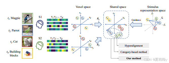
for 2 subjects with the same stimuli, existing works mapping the fMRI signals to voxel space. Then aggregate/cluster the fMRI signals with the same stimuli. However, it is hard to generalize. So another method clusters each categories.

2.3. Methodology

2.3.1. Overview

        ①Overall framework:

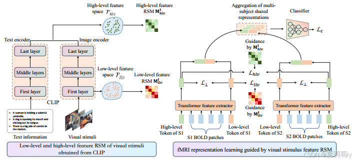
        ②: voxel space

        ③: the neural responses of the -th subject in total , where  is the number of image stimuli and  is the number of voxels（那为什么不是）

        ④: pixel space of image stimuli

        ⑤: label space of image stimuli

        ⑥Classifier: 

2.3.2. CLIP-based feature extraction of visual stimuli

        ①They extract low-level feature and high level feature by the first layer of image encoder and the average value of the last layer of the whole CLIP (image and text encoder)

        ②Representation similarity matrices (RSMs)  and  is to quantify the similarity between  (batch size) visual stimuli in low-level and high-level feature spaces.  and  in  and  denote image similarity in  and 

2.3.3. Transformer-bsed fMRI feature extraction

        ①Transformer process:

        ②Transformer-based fMRI feature extractor:

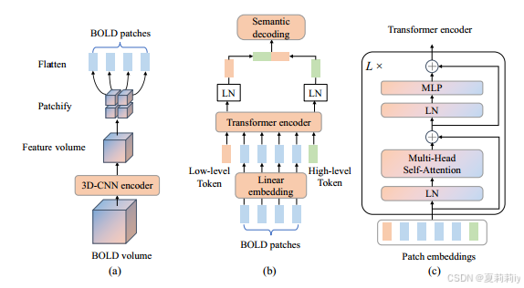
(a) they firstly reduce the dimension of BOLD volume and then patchify and flatten them, functions of (b) and (c) are:

2.3.4. Multi-subject shared neural response representation

        ①Similarity loss:

2.3.5. Semantic classifier

        ①Final representation:

        ②Semantic classification CE loss:

2.3.6. Optimization objective

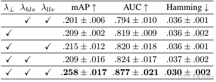
        ①Orthogonal constraint to encourage the difference between low-level and high-level token representations:

        ②Final loss:

2.4. Experiments

2.4.1. Datasets

（1）HCP

        ①Subjects: 9 of 158

        ②Visual stimuli: four dynamic movie clips, each annotated with an 859-dimensional WordNet label

        ③Categories: labels which frequency higher than 0.1

（2）NSD

        ①Subjects: 8

        ②Visual stimuli: MSCOCO, each image has multiple labels from 80 categories. Different 9k stimulus for each subject and the same 1k for all the subjects

2.4.2. Baseline methods

        ①Types of compared methods: Single-subject decoding methods, multi-subject data aggregation methods, MS-EMB, Shared response model (SRM)

2.4.3. Parameter settings

（1）HCP

        ①3D-CNN: 6 layers, obtaining 7×8×7×512, and reshape to 392×512 (359 patches)

        ②Transformer blocks: 2

        ②Optimizer: Adam with 0.001 learning rate

        ③Batch size: 64

        ④Hyperparameter of loss weights: 

（2）NSD

        ①Embedding layers: 512, 24

        ②Head: 8

        ③Batch size: 64

        ④Optimizer: Adam with 0.0001 learning rate

        ⑤Hyperparameter of loss weights: 

2.4.4. Evaluation metrics

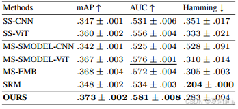
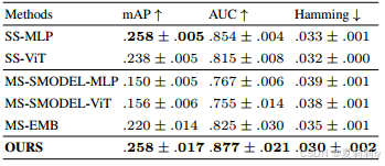
        ①Mean Average Precision (mAP), the area under the receiver operating characteristic curve (AUC) and Hamming distance

2.4.5. Comparative experimental results

        ①Performance on HCP:

        ②Performance on NSD:

2.4.6. Ablation study

        ①Loss ablation:

2.4.7. Visualization

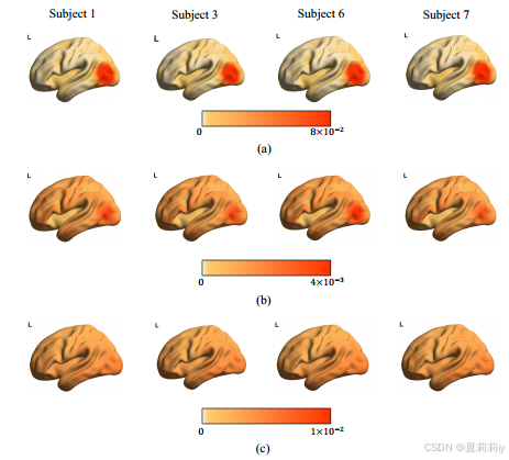
        ①(a) low-level tokens, (b) high-level tokens, (c) attention map of MS-EMB method:

2.5. Discussion and Conclusion

        ~